Encoding Intuitions

Discipline before cleverness.

Burned by Intuition

Actuaries are clever people, and they model lots of things intuitively. For example, an actuary might have two models with different data or methods trying to estimate the same phenomenon. Under model X they get an estimate of 5%, and under model Y they get an estimate of 8% (They're actuaries, so it's likely an Excel spreadsheet and only point estimates, sadly). However, the actuary trusts the data in model X more than in Y, so they use their actuarial judgment, hunch, prior, best guess, or intuition to weight X and Y by 80%/20% to get 5.6%.

But intuition can fail us. Consider this Richard McElreath variation on the Monty Hall problem:

Someone is cooking pancakes. They have to calibrate the stove temperature, and as a result, the first three pancakes come out like this:

1. Burned on both sides
2. Burned on one side, perfect on the other
3. Perfect on both sides

You are served a pancake, and you only know the top side is burned. What is the probability that the other side is also burnt?

The common intuition is that you must have one of the two pancakes with a burnt side, so 1/2. But this is wrong.

I frequently see actuaries do things that seem intuitive, but how often is it wrong and goes unnoticed? A better way to conduct ourselves would be to be disciplined and use formal models when available. Thus, let me formally introduce you to Bayes theorem.

Bayes' theorem is a framework for updating our beliefs in light of new evidence.

Bayes' Theorem

$$
P(H \mid E) = \frac{P(E \mid H) \cdot P(H)}{P(E \mid H) \cdot P(H) + P(E \mid \neg H) \cdot P(\neg H)}
$$

• \( P(\cdot) \): Probability of an event.
• \( H \): Prior hypothesis or belief before seeing evidence.
• \( E \): Evidence or new data observed.
• \( P(E \mid H) \): Likelihood of observing evidence \( E \) given the hypothesis \( H \).
• \( P(H \mid E) \): Posterior probability, updated belief, hypothesis, or estimate after considering the new evidence.
• \( P(\neg H) \): Probability that the hypothesis is false. Which is the compliment to the hypothesis being true so that they add up to 1.00.

The denominator \( P(E) \) represents the total probability of observing the evidence under all scenarios, if the hypothesis true or false:

$$
P(E) = P(E \mid H) \cdot P(H) + P(E \mid \neg H) \cdot P(\neg H)
$$

This ensures that the posterior probability \( P(H \mid E) \) is properly normalized between 0 and 1.

Returning to the pancakes (which, unfortunately, are cold now), we can use Bayes theorem to calculate the probability that the bottom side is also burnt, given we see the top side is burnt.

\( P(H) = 0.33 \): Probability that both sides are burnt. This occurs for one of the three pancakes.

\( P(\neg H) = 1 - P(H) = 0.66\): Probability that both sides are not burnt.

\( E \): Evidence, after observing that the top side is burnt.

\( P(E \mid H) = 1.00 \): Probability of seeing a burnt top side if we have the double-burnt pancake (both sides burnt).

Next, we compute the total probability of observing the evidence \( P(E) \), and we need \( P(E \mid \neg H) = 0.25\): Probability of observing a burnt side if it's not the double-burnt pancake. One of the four remaining sides is burnt.

Now substitute the values:

$$
P(E) = [P(E \mid H) \cdot P(H)] + [P(E \mid \neg H) \cdot P(\neg H)]
$$

$$
P(E) = [1.00 \cdot 0.33] + [0.25 \cdot 0.66] = 0.495
$$

Substitute the values:
$$
P(H \mid E) = \frac{1.00 \cdot 0.33}{0.495} = 0.67 \quad \text{(or } \frac{2}{3}\text{)}
$$

There's a 2/3 chance of having the burnt pancake on both sides; not 1/2. It's not intuitive.

The Full Enchilada

Here's another example showing how Bayesian inference can extend from point estimates to distributions. But first, a simplified Bayes theorem:

$$ Posterior \propto Likelihood \times Prior $$

$$ p(H \mid E) \propto p(E \mid H) \times p(H) $$

This form may appear different from the previous version, and the symbol \( \propto \) means "proportional to." Calculating \( p(E) \) algebraically can be impractical, making it easier to work with this simplified version. Computer simulations to sample posterior distributions can take advantage of this version, too, but we won't go into the details.

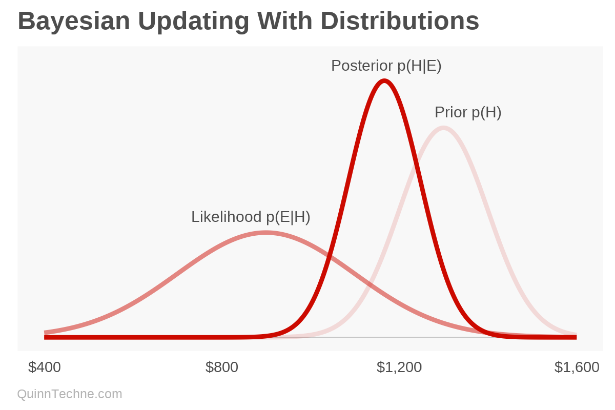
How does it work? Suppose an actuary is forecasting the annual cost of something. They assume it is normally distributed (Gaussian or bell-shaped) with a mean of $1,300 and a standard deviation of ±$100. This is their prior.

The actuary then gets two data points: quarterly costs. They assume these costs also come from a normal distribution. After annualizing the costs and adjusting for inflation to the forecast period, the actuary has $950 and $850, believing they have a standard deviation of ±$200. You encode your uncertainty in the variance, precision, volatility, spread, or standard deviation. The actuary is less certain from a quarter's worth of data versus an annual forecast—think Central-limit theorem and the square root relationship of standard deviation to sample size.

• Prior: Normal($1,300, ±$100)
• Likelihood: Normal(E, ±$200)
• E, evidence, or new data: $950, $850
• Posterior: wait for it...

• Posterior: Normal($1,167, ±$82)

We started with our prior of $1,300 and have a new average of $1,166 after seeing the new data. Bayesian updating, ta-da!

Calculating Posteriors

So, how can one calculate these? Here are a few examples in R. Setting up these R methods usially requires free software besides R, like Rtools, Stan, or JAGS. We are going to use the same numbers as the chart, which means we're updating our prior, the mean, which is called mu (μ). First, we'll look at quap(), which approximates the posterior distribution, making it very fast. It is part of the rethinking package, and the example shows the slim version which requires no extra software. Then we'll look at rjags and cmdstanr which use a simulation method called Markov chain Monte Carlo (write that down, it'll be on quiz at the end). Last, we'll show brms which is also Stan, but written like a vanilla R regression model.

quap

# Install quap()
# install.packages(c("coda","mvtnorm","devtools","loo","dagitty"))
# devtools::install_github("rmcelreath/rethinking@slim")

library(rethinking)

# Model
flist <- alist(
    new_data ~ dnorm(mu, 200), # Likelihood with known standard deviation
    mu ~ dnorm(1300, 100) # Prior
  )
  
new_data <- data.frame(new_data = c(950, 850))

# Fit the model
mod_quap <- quap(flist, data = new_data) 

> precis(mod_quap) # Posterior distribution
      mean    sd    5.5%   94.5%
mu 1166.67 81.65 1036.17 1297.16

JAGS

library(rjags)

# Model
# Note that the syntax uses precision (1/sigma^2) instead of variance (sigma^2)
model_string <- "
  model {
    for (i in 1:N) {
      new_data[i] ~ dnorm(mu, 1/(sigma^2)) 
    }
    mu ~ dnorm(1300, 1/(100^2))
    sigma <- 200
  }
"

data_jags <- list(new_data = c(950, 850), N = 2)

# Fit model
model_jags <- jags.model(
  textConnection(model_string),
  data = data_jags,
  n.chains = 4,
  n.adapt = 500
)

parameters <- c("mu")

# Sample posterior
samples_jags <- coda.samples(
  model_jags,
  variable.names = parameters,
  n.iter = 4000
)

> summary(samples_jags) # Posterior distribution

Iterations = 1:4000
Thinning interval = 1 
Number of chains = 4 
Sample size per chain = 4000 

1. Empirical mean and standard deviation for each variable,
   plus standard error of the mean:

          Mean             SD       Naive SE 
     1167.1296        82.2417         0.6502 
Time-series SE 
        0.6502 

2. Quantiles for each variable:

 2.5%   25%   50%   75% 97.5% 
 1007  1111  1168  1222  1327 

Stan

# Loading Stan
library(cmdstanr)
cmdstan_path()
cmdstanr::check_cmdstan_toolchain(fix = TRUE)
set_cmdstan_path(path = 'c:\\cmdstanr\\cmdstan-2.35.0') # System dependent

options(
  mc.cores = parallel::detectCores(),
  stanc.allow_optimizations = TRUE,
  stanc.auto_format = TRUE
)

# Model
code_stan <- write_stan_file(
  "data {
    int <lower=0> N;         
    array [N] real new_data; //Object, size, variable type, variable name
  }
  
  parameters {
    real mu; 
  }
  
  model {
    mu ~ normal(1300, 100);          // Prior
    new_data ~ normal(mu, 200);      // Likelihood
  }"
)

# Compile model
mod_check <- cmdstan_model(code_stan, compile = FALSE)  
mod_check$check_syntax()
mod <- cmdstan_model(code_stan, pedantic = TRUE, dir = 'c:\\cmdstanr')  

data_stan <- list(N = 2, new_data = c(950, 850))

# Fit and sample
fit <- mod$sample(
  data = data_stan,
  iter_warmup = 200,
  iter_sampling = 4000,
  chains = 4
)  

> fit$print() # Posterior distributions
  variable    mean  median    sd   mad      q5     q95 rhat ess_bulk ess_tail
     lp__   -3.24   -2.95  0.74  0.31   -4.73   -2.73 1.00     7283     8344
     mu   1167.49 1167.50 82.52 80.95 1031.28 1305.12 1.00     5715     7700

brms

library(brms)

new_data <- c(950, 850)

# Create a  formula that uses the known standard deviation
brms_formula <- bf(new_data ~ 1, sigma = 200) # Likelihood

# brms model
mod_brms <- brm(
  formula = brms_formula,                          
  data = data.frame(new_data = new_data), 
  family = gaussian(), 
  prior = c(
    prior(normal(1300, 100), class = "Intercept") # Prior 
  ),
  chains = 4,                           
  iter = 4000,                          
  warmup = 200  
)

> summary(mod_brms)
 Family: gaussian 
  Links: mu = identity; sigma = identity 
Formula: new_data ~ 1 
         sigma = 200
   Data: data.frame(new_data = new_data) (Number of observations: 2) 
  Draws: 4 chains, each with iter = 4000; warmup = 200; thin = 1;
         total post-warmup draws = 15200

Regression Coefficients:
          Estimate Est.Error l-95% CI u-95% CI Rhat Bulk_ESS Tail_ESS
Intercept  1166.59     82.95  1000.78  1326.43 1.00     6013     7822

Further Distributional Parameters:
      Estimate Est.Error l-95% CI u-95% CI Rhat Bulk_ESS Tail_ESS
sigma   200.00      0.00   200.00   200.00   NA       NA       NA

This is a simple Bayesian model calculated four different ways. In all cases, the posterior distribution of mu, the updated mu given the data, is around 1,166. Yet, this simplicity can easily extend into powerful regression and time series models. These more complex models come with comprehensive workflows, model diagnostic, and best practices, but we'll save those for another day.

Because, Excel

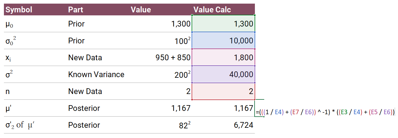
Wait! I'm an actuary, and I'm only comfortable with Excel. Please, please show me how to do this in Excel! Okay, fine. But you didn't learn this from me.

You can algebraically solve some types of posteriors. This example we're using is a known variance case, so you can use a normal-normal conjugate update. We'll use the formulation from Wikipedia.

The posterior update for \( \mu \), given data \( x_i \) and assuming a normal likelihood with known variance \( \sigma^2 \), is given by:

• Prior: \( \mu_0 \), with variance \( \sigma_0^2 \)
• Posterior: Updated \( \mu' \), with the posterior variance

The posterior update formula is:

$$
\mu' = \left( \frac{1}{\sigma_0^2} + \frac{n}{\sigma^2} \right)^{-1} \left( \frac{\mu_0}{\sigma_0^2} + \frac{\sum_{i=1}^{n} x_i}{\sigma^2} \right)
$$

Where:

• \( \mu_0 \): mu (the subscript is sometimes pronounced "nought") is the prior mean.
• \( \sigma_0^2 \): sigma nought is the prior variance.
• \( x_i \): are the observed data points.
• \( \sigma^2 \): is the known variance of the data likelihood.
• \( n \): is the number of observed data points.
• \( \mu' \): is the updated posterior mean.

Here's how it comes together.

And how does this posterior average compare to other results?

Weighty Jargon

Communicating Bayesian concepts can be confusing for most audiences. But, if your credibility is ever in a pinch, just say "posterior predictive distribution," and like abracadabra! you're credible again. Or, you can also compute an implied weighting between your original (prior) value, new data, and result (posterior) and communicate that instead. For example:

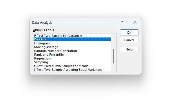
Weight on prior data: 66.6% (It's just coincidence—you wanted the dark arts!)

$$
66.6\% \times 1300 + 33.4\% \times \left( \frac{950 + 850}{2} \right) = 1167
$$

The implied weight is a function of our uncertainty encoded in our prior or likelihood. In this example, only the Likelihood changes. A smaller standard deviation means you trust the new evidence more and more weight would be given to the new data. A larger standard deviation means more uncertainty and thus less weight on the new evidence. This relation goes for the standard deviation on your prior, too.

Encoding Intuitions

Bayesian models offer an intentional and transparent way to update our forecasts based on new data. So, when it's time to integrate new evidence (or send your pancake back to the chef), consider making the formal calculation—your conclusions will be all the more disciplined for it.

McElreath, R. (2020). Statistical Rethinking: A Bayesian Course with Examples in R and Stan (2nd edition). Chapman and Hall/CRC. https://xcelab.net/rm/

Wikipedia contributors. (2024). Conjugate prior. In Wikipedia, The Free Encyclopedia. https://en.wikipedia.org/wiki/Conjugate_prior

Calculations and graphics done in R version 4.3.3, with these packages:

Chang W, Cheng J, Allaire JJ, Sievert C, Schloerke B, Xie Y, Allen J, McPherson J, Dipert A, Borges B (2024). shiny: Web Application Framework for R. R package version 1.9.1. https://CRAN.R-project.org/package=shiny

McElreath R (2024). rethinking: Statistical Rethinking book package. R package version 2.40. https://github.com/rmcelreath/rethinking

Plummer M, Stukalov A, Denwood M (2024). rjags: Bayesian Graphical Models using MCMC. R package version 4-16. https://CRAN.R-project.org/package=rjags

Qiu Y (2024). showtext: Using Fonts More Easily in R Graphs. R package version 0.9-7. https://CRAN.R-project.org/package=showtext

Stan Development Team (2024). cmdstanr: R Interface to CmdStan. R package version 0.7.0. https://mc-stan.org/cmdstanr/

Wickham H, et al. (2019). Welcome to the tidyverse. Journal of Open Source Software, 4 (43), 1686. https://doi.org/10.21105/joss.01686

This website reflects the author's personal exploration of ideas and methods. The views expressed are solely their own and may not represent the policies or practices of any affiliated organizations, employers, or clients. Different perspectives, goals, or constraints within teams or organizations can lead to varying appropriate methods. The information provided is for general informational purposes only and should not be construed as legal, actuarial, or professional advice.