Uniform documentation.
Underwriting
An Underwriting margin component is required in Medicaid capitation rates per 42 CFR § 438.5(e). The underwriting margin ratio is akin to net income, or net margin. Until 2019, there was no widely known attempt to externalize the process of calculating it for Medicaid rates. Then, the Medicaid Health Plans of America (MHPA) published a model. Part of the model relied on an assumption of how much the net margin ratios varied. This post explores the estimation or fitting of that parameter.
The MHPA model fits potential net income ratios. With some inclusion criteria, they used post-tax health plans' net income data from 2013–2015, which was collected and reported by the Society of Actuaries in 2017.
The documentation uses the following model to fit the variance, or the standard deviation parameter denoted sigma (σ).
$$
y_i \sim \mathcal{N}\bigl(\theta_{j[i]},\sigma_i\bigr)
$$
$$
\theta_{j[i]} \sim 0.5 \times \mathcal{N}(0.010,0.002)+0.5 \times \mathcal{N}(0.020,0.002)
$$
$$
\sigma_i =\sqrt{\alpha+\frac{\omega}{\text{member_months}_i}}
$$
$$
\alpha \sim \text{Uniform}(0,M_\alpha)
$$
$$
\omega \sim \text{Uniform}(0,M_\omega)
$$
- \( y_i \): Observed net income ratio for observation \(i\), where \(i\) is the unique combination of health plan, state, and year.
- \( \theta_{j[i]} \): Random mean for observation \(i\), drawn from a 50/50 mixture of two normals distributions (or Gaussian with mean and standard deviation).
- \(j\): State \(j\).
- \([i]\): Year associated with observation \(i\).
- \( \sigma_i \): Standard deviation for observation.
- \( \alpha \): Irreducible variance parameter,
alpha. - \( \omega \): Reducible variance parameter,
omega. - \( M_\alpha, M_\omega \): Upper bounds on uniform priors for \(\alpha\) and \(\omega\), respectively. The documentation does not specify the upper bound; we will use 10,000.
For context, a member month is a common way to describe the size of a health plan. It is an exposure measure. For example, if person A joins a health plan and stays all year, they generate 12 member months. If person B joins in January and leaves at the end of October, they generate 10 member months.
The model has three interesting features. First, historical net incomes are modeled as clustering around 1% and 2%. When I wrote about Medicaid underwriting gains, I found similar clustering: around 0% and 2% for underwriting gain ratios.
Second, the model assumes an ambient amount of volatility in alpha and a reducible amount omega. Think of the central limit theorem and how the means of larger samples have less variance than the means of smaller samples.
Last are the uniform priors. The model documentation says they're uniform but without specifying the range. Selecting a model, and explicitly priors, is a way to encode background information about the topic. alpha and omega are related to a standard deviation, so it's unlikely they're less than zero at their lower bound. But the upper bound? Undocumented. Weakly informative priors are preferred to the rigidness of uninformative or uniform ones.
Codewriting
Let's try to replicate this model and the results with R and Stan. We'll start with importing the data MHPA kindly provided in the worksheet "Table 1 - MCO Margin Data" and looking at state-specific net income (net_margin) statistics (Managed Care Organization, or MCO, is a common term for a Medicaid health insurer or health plan):
> glimpse(mco_data)
Rows: 230
Columns: 8
$ state                <chr> "AZ", "AZ", "AZ", "AZ", "AZ", "AZ"…
$ corporate_mco_name   <chr> "UnitedHealth Group Inc.", "Aetna"…
$ local_mco_name       <chr> "Arizona Physicians IPA", "Mercy C…
$ year                 <dbl> 2015, 2015, 2015, 2015, 2015, 2015…
$ is_medicaid_dominant <dbl> 1, 1, 1, 1, 1, 1, 1, 1, 1, 1, 1, 1…
$ member_months        <dbl> 4756644, 4011096, 2763600, 1630440…
$ revenue              <chr> "N/A", "N/A", "N/A", "N/A", "N/A",…
$ net_margin           <dbl> 0.023600000, 0.003393821, 0.029268…

state_summary <- mco_data |>
  group_by(state) |>
  summarize(
    mean_net_margin = round(100 * mean(net_margin), 1),
    sd_net_margin = round(100 * sd(net_margin), 1),
    median_mms = median(member_months),
    n = n(),
    .groups = 'drop'
  ) |>
  filter(n > 1) |>
  arrange(state) |>
  print(n = 100)

# A tibble: 33 × 5
   state  mean_net_margin  sd_net_margin    median_mms     n
   <chr>     <dbl>            <dbl>              <dbl>   <int>
1  AZ         1.9              6.3             1251348     9
2  DC         1.7              3.8              389475     9
3  FL        -5.9              6.6              489934     5
4  GA         2.0              1.7             4062898     5
5  IA        -5.1              2.9              691900     3
6  IL        -2.1              7.2              415146     9
7  IN         0.7              1.3             3417155     3
8  KS        -2.8              7.1             1415523     6
9  KY         6.6              4.9             1187320     6
10 LA        -0.3              2.6             1747182    10
11 MA         7.8              4.5              565620     3
12 MD         0.6              4.8             2658970     5
13 MI         1.7              4.2              767100    29
14 MN         0.1              3.5             1271414     2
15 MO        -0.2              5.2             1155023     9
16 MS        -1.2              2.7              925642     5
17 NE        -1.2              3.0              272101     3
18 NH        -4.8              1.3              565313     3
19 NJ         1.7              4.4             2150453     7
20 NM         1.2              2.2             1012031     7
21 NV         3.0              1.1             1722877     3
22 OH         2.9              3.4             2729938    15
23 OR        -0.3              5.3              364182     2
24 PA         0.8              1.8             2127744    11
25 RI         1.4              2.0             1651053     3
26 SC         1.9              3.4             1253641    12
27 TN         2.6              0.7             4759718     6
28 TX         0.6              4.9             1405661    15
29 UT        -1.6              5.8               95992     2
30 VA         0.3              2.3              706089     5
31 WA        -0.7              2.5             1679396     6
32 WI         5.9              6.5             1533902     6
33 WV         4.0              4.0             1049520     4
Based on this prior output, let's look at some plots. We can get a sense of the distribution of net margin standard deviations by plotting it by year:
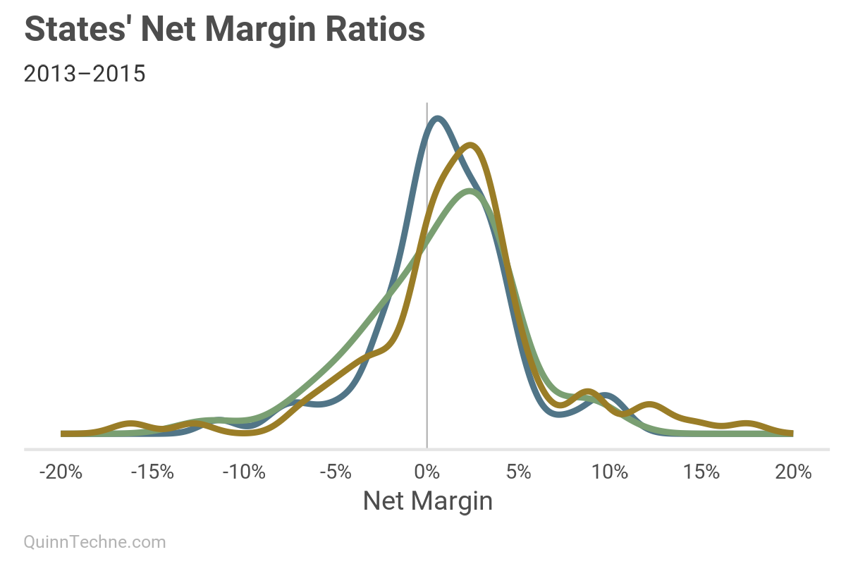
Notice how the peaks, or statistical modes, are right of 0%. On average, a health plan can expect a positive net margin for putting their capital at risk (good!). Another way to explore the net margin is to chart the distribution of states' standard deviations of the net margin. Think of it as all states' possible sigmas, σ, and how often they occurred in the data:
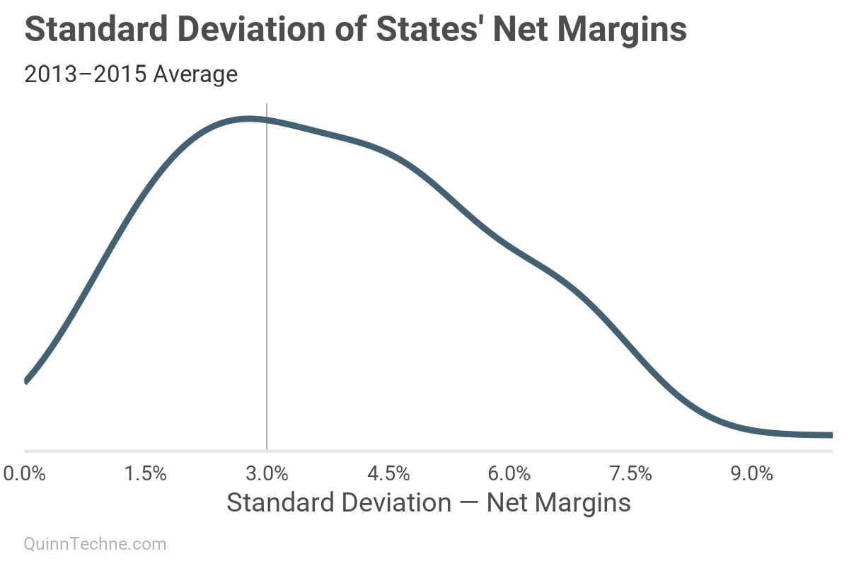
It seems the peak is a little less than 3%, and there's a lot of area to the right of 3%, too, suggesting an average deviation higher than that. This next look will support our hypothesis that increasing member months reduces the standard deviation.
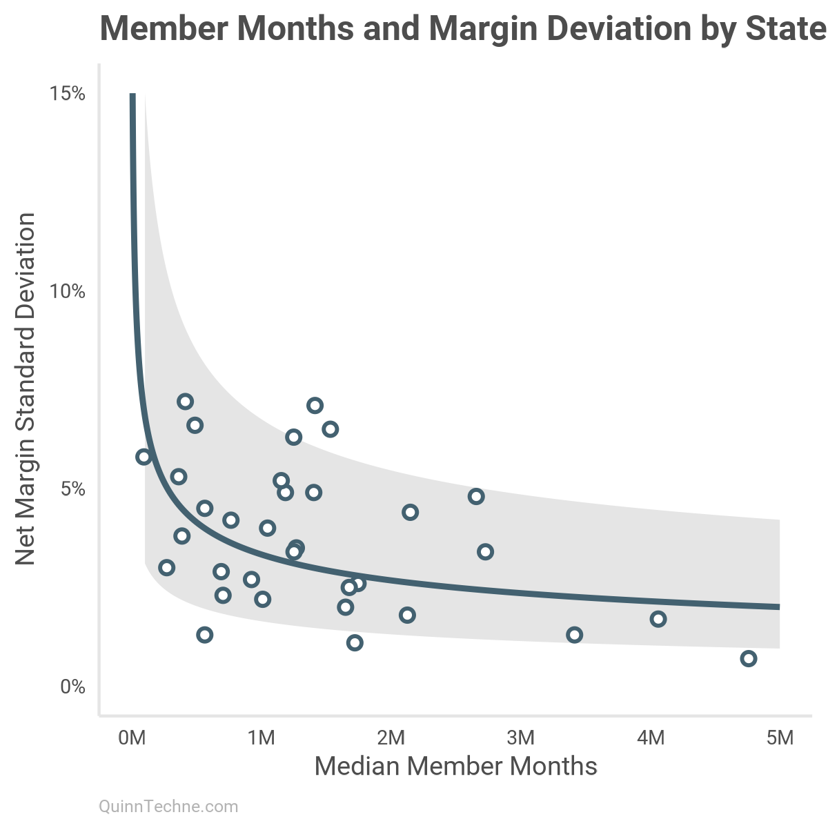
The negative slope suggests the relationship holds.
Given the model documentation and formula I outlined, this Stan model is my best interpretation of the model. The documentation was unclear about just how wide the uniform prior was for alpha and omega, which ends up being important later.
data {
  int <lower = 1> N;
  int <lower = 1> states;
  int <lower = 1> years;
  array[N] int <lower = 1, upper = states> state;
  array[N] int <lower = 1, upper = years> year;
  vector[N] net_margin;
  vector <lower = 1> [N] member_months;
}

parameters {
  matrix[states, years] mu;
  real <lower = 0> alpha;
  real <lower = 0> omega;
}

transformed parameters {
  vector[N] sigma;

  for (n in 1:N) {
    sigma[n] = sqrt(alpha + omega / member_months[n]);
  }
}

model {
  for (j in 1:states) {
    for (t in 1:years) {
      target += log_mix(
        0.5,
        normal_lpdf(mu[j, t] | 0.01, 0.002),
        normal_lpdf(mu[j, t] | 0.02, 0.002)
      );
    }
  }

  alpha ~ uniform(0.0, 10000);
  omega ~ uniform(0.0, 10000);

  for (n in 1:N) {
    net_margin[n] ~ normal(mu[state[n], year[n]], sigma[n]);
  }
}

generated quantities {
  vector[N] y_rep;
  for (n in 1:N) {
    y_rep[n] = normal_rng(mu[state[n], year[n]], sigma[n]);
  }

  vector[N] log_lik;
  for (n in 1:N) {
    log_lik[n] = normal_lpdf(net_margin[n] | mu[state[n], year[n]], sigma[n]);
  }
}
Notice how Stan models are in blocks:
- data
- parameters
- transformed parameters
- model
- generated quantities
Stan forces you to code all model parts explicitly. While a pain to debug, the specificity is valuable in concretizing your conception of the model. Moreover, you can start encoding your intuitions before a tool forces you.
Mixed distributions can be odd in Stan. The mathematical formula feels straightforward compared to the more complex code of specifying log densities. The index j is for state, and t is for year:
for (j in 1:states) {
    for (t in 1:years) {
      target += log_mix(
        0.5,
        normal_lpdf(mu[j, t] | 0.01, 0.002),
        normal_lpdf(mu[j, t] | 0.02, 0.002)
      );
    }
  }
With the model coded, we can start to sample from the posterior and look at some model diagnostics. We'll sample 4,000 times like the MHPA model.
### Stan compile
mod_check <- cmdstan_model(stan_code_1, compile = FALSE)
mod_check$check_syntax()
stan_mod_1 <- cmdstan_model(stan_code_1, pedantic = TRUE, dir = 'c:\\system_specific')
### Stan input
stan_mod_list_1 <- list(
  N = nrow(mco_data),
  states = length(unique(mco_data$state)),
  years = length(unique(mco_data$year)),
  state = as.numeric(factor(mco_data$state)),
  year = as.numeric(factor(mco_data$year)),
  net_margin = mco_data$net_margin,
  member_months = mco_data$member_months
)
### Stan Fit
stan_fit_1 <- stan_mod_1$sample(
  data = stan_mod_list_1,
  init = list(
    list(alpha = 0.02, omega = 0.02),
    list(alpha = 0.02, omega = 0.02),
    list(alpha = 0.02, omega = 0.02),
    list(alpha = 0.02, omega = 0.02)
  ),
  set.seed(20250220),
  iter_warmup = 4000,
  iter_sampling = 4000
)
Bayesian model diagnostics, for models fit by software like Stan or rjags, include checking chain convergence (trace plots, \( \hat{R} \), effective sample sizes), performing posterior predictive checks, and using information criteria (e.g., leave-one-out cross-validation) to confirm the model has converged and fits the data adequately.
For this model, we'll focus on a few diagnostics. Rest assured, the convergence and trace plots look good for all parameters.
Let's first look at the pairs plot of alpha and omega:
mcmc_pairs(stan_fit_1$draws(), regex_pars = "^(alpha|omega)$")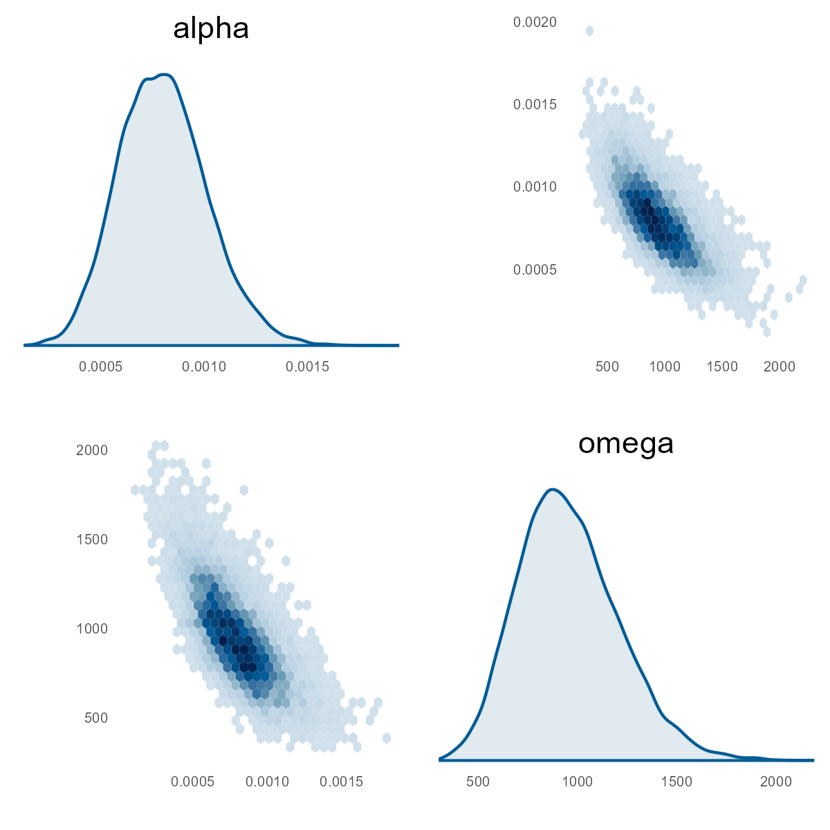
The distribution shows the magnitude of the parameters. Looking at alpha, it is similar to the MHPA model. Let's look at the difference between this fit versus MHPA. In this next chart, we get the distribution of the differences in alpha, which shows we measure similarly given the probability mass around zero difference.
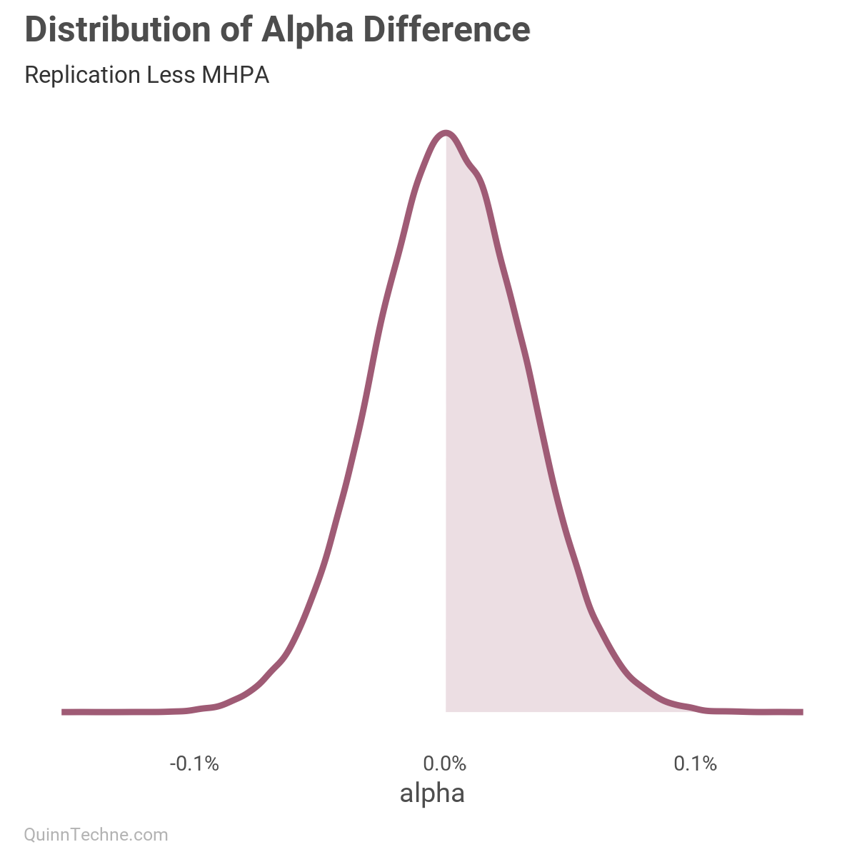
Back to the blue pairs plots, let's look at omega. In the MHPA model, this value is 0.0008–0.0011. From the pairs plot, we see the replication values at 725–1,050. Wow! What is going on?
First, the data might have been supplied incorrectly. Two, somewhere in my process, I failed to replicate the same filtering or Stan model. My suspect would be the uniform priors, as the MHPA model doesn't say what uniform interval they used. Perhaps the MHPA uniform priors had a smaller maximum for a total range of [0.00, 0.05]. Or, we're both doing something wrong.
A mean MHPA omega value of 0.0956% is odd, given that alpha is similar in magnitude at 0.0782%. Remember, the formula is that omega is reducible by member months. Two member months and omega is halved:
- 1 member month: \( \sqrt{0.0782\% + \frac{0.0956\%}{1}} = 4.2\% \)
- 2 member months: 3.6%
- 12 member months: 2.9%
- 50,000 member months: 2.8%
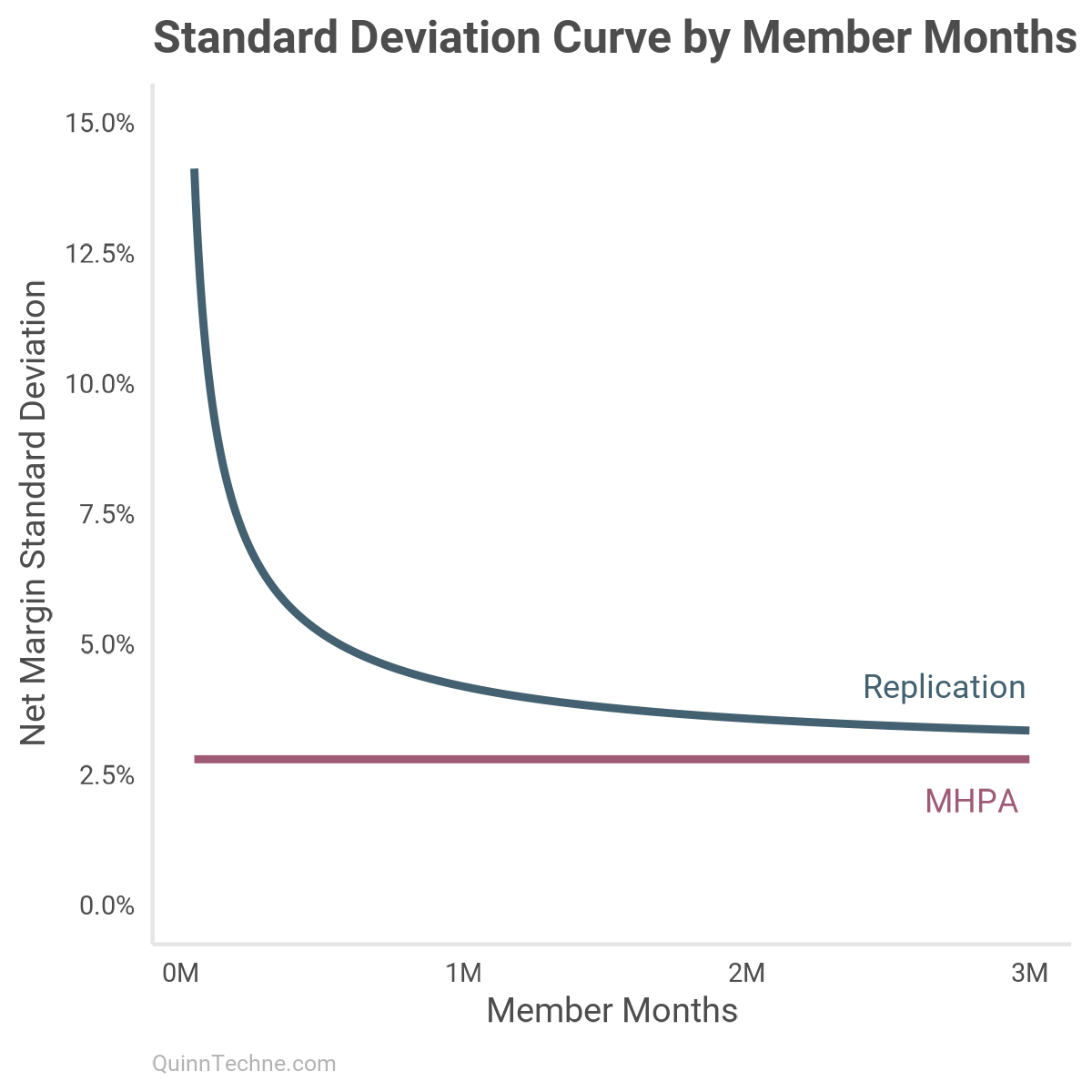
The model documentation says the data is filtered to observations with at least 50,000 member months. In that case, why even have omega that small? The model could be fit with just alpha. Here is the standard deviation charted from 50,000 to 3 million member months between the replication model (blue) and MHPA (maroon):
But is the replication model functionally the same as the MHPA one? One way to look at their performance is to have the model make predictions (y_rep) and compare it to the observed data (y). These are called posterior predictive checks. For the MHPA checks, it is the same prior Stan code for the replication model, but alpha and omega have been replaced by very tight priors around the mean MHPA values. This is the Stan model change:
  alpha ~ normal(0.0008, 0.00001);
  omega ~ normal(0.0010, 0.00001);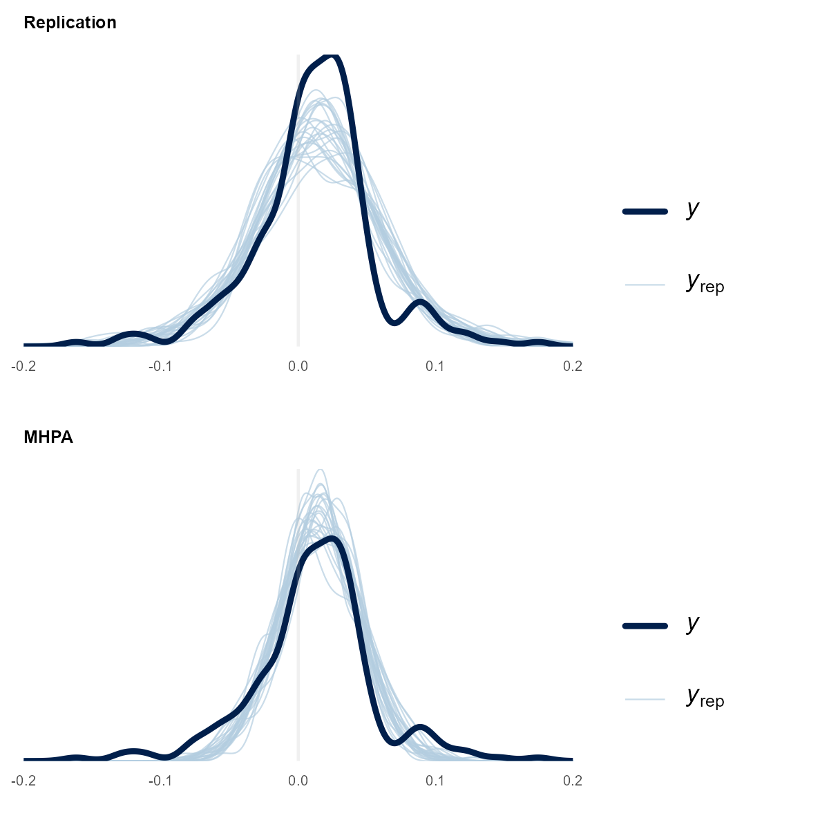
In the prior plots, we can see the replication model lacks the peak but fits the tails. The MHPA model is the opposite: more in the peak and smaller tails. Investigating the bump at 0.1 net margin could lead to new model ideas (but not today).
Another way to assess a Stan model fit is with the expected log pointwise predictive density (ELPD). It measures model out-of-sample predictive accuracy. We can compare accuracies across these models where higher ELPD values indicate better predictive performance.
 #                            Estimate    SE
 # elpd_loo1 Replication (1)   393.5    22.1
 # elpd_loo2 MHPA (2)          205.6    46.4

> loo_compare(
+ loo(stan_fit_1$draws("log_lik")),
+ loo(stan_fit_2$draws("log_lik"))
+ )
       elpd_diff  se_diff
model1      0.0      0.0
model2    -87.9     32.8
In this case, the replication model performs better, given the difference is about 2.7 stand errors between models.
Is the model difference practically different? For a health plan of size 1 million member months, the net margin standard deviations would be:
- Replication model: 4.2%
- MHPA model: 2.8%
The smaller MHPA number might be understating the financial risk health plans face. The forecasted risk of a net margin ≤-4% goes from odds of 1:10 in the replication model to 1:60 under MHPA. Plan accordingly.
Origins
I am fond of the MHPA model. When it was new in 2019, and I read its documentation, its section about parameter fitting rekindled my interest in Bayesian statistics. The next year I signed up for Dr. Matthew Heiner's Coursera class, which led to what I write about now.
With this all said, I have not seen the MHPA model in circulation. The documentation is easy enough to find, but the Excel model cannot be found (I happened to have an old email attachment of it). This end might be fine because its most valuable contribution was instigating the Society of Actuaries to build its underwriting margin model in 2022.
We'll investigate how the Society of Actuaries fits its variance parameters in part II.
Gelman, A., Carlin, J. B., Stern, H. S., Dunson, D. B., Vehtari, A., & Rubin, D. B. (2013). Bayesian Data Analysis (3rd edition). Chapman and Hall/CRC.
Gibson, S. H., Piekut, J. R., Simons, J. (2019). Underwriting Gain Development for Managed Medicaid Capitation Rates. MHPA. https://medicaidplans.org/wp-content/uploads/2020/07/MHPA-Underwriting-Gain-Development-Report_June-2019_FINAL.pdf. The Excel file was called "MHPA Underwriting_Gain_Model_6.14.19_excel_.xlsb".
Society of Actuaries (2017). Medicaid Managed Care Organizations: Considerations in Calculating Margin in Rate Setting. https://www.soa.org/globalassets/assets/Files/Research/medicaid-managed-report.pdf
Calculations and graphics done in R version 4.3.3, with these packages:
Auguie B. (2017). gridExtra: Miscellaneous Functions for "Grid" Graphics. R package version 2.3. https://CRAN.R-project.org/package=gridExtra
Carr D, Lewin-Koh N, Maechler M, Sarkar D (2024). hexbin: Hexagonal Binning Routines. R package version 1.28.5. https://CRAN.R-project.org/package=hexbin/
Gabry J, Mahr T (2024). bayesplot: Plotting for Bayesian Models. R package version 1.11.1. https://mc-stan.org/bayesplot/
Stan Development Team (2024). cmdstanr: R Interface to CmdStan. R package version 0.7.0. https://mc-stan.org/cmdstanr/
Qiu Y (2024). showtext: Using Fonts More Easily in R Graphs. R package version 0.9-7. https://CRAN.R-project.org/package=showtext
Vehtari A, Gabry J, Magnusson M, Yao Y, Bürkner P, Paananen T, Gelman A (2024). loo: Efficient leave‑one‑out cross‑validation and WAIC for Bayesian models. R package version 2.8.0. https://mc-stan.org/loo/
Wickham H, et al. (2019). Welcome to the tidyverse. Journal of Open Source Software, 4 (43), 1686. https://doi.org/10.21105/joss.01686
This website reflects the author's personal exploration of ideas and methods. The views expressed are solely their own and may not represent the policies or practices of any affiliated organizations, employers, or clients. Different perspectives, goals, or constraints within teams or organizations can lead to varying appropriate methods. The information provided is for general informational purposes only and should not be construed as legal, actuarial, or professional advice.

