State it explicitly.
Underwriting Again
In Part I, we examined fitting the standard deviation (SD) parameter of net margin ratios from the Medicaid Health Plans of America (MHPA) Underwriting Gain Development model. The result was an exposure-sensitive SD that did not align between the original and replication models.
For part two, we'll look at the Society of Actuaries' (SOA) subsequent underwriting margin model published three years later in 2022. It uses an underwriting ratios (UWR) distribution as part of the model. Net margins in the MHPA model are different from UWRs yet highly positively correlated.
The latest SOA model, updated in 2024, uses 2013–2022 UWR data by year, state, and health plan from the National Association of Insurance Commissioners (NAIC) Annual Health Statements. Like MHPA, the data is similarly filtered to plans with at least 50,000 member months plus other inclusion criteria. The data and model documentation are available on the SOA website.
The data here is from the workbook 2024 "margin-model-data-backup.xlsm" and a combination of the main data on the worksheet [Figure 1 and 2] with the state variable joined by health plan IDs from [S&P extract 240118].
> glimpse(soa_data)
Rows: 1,899
Columns: 18
$ year                          <dbl> 2013, 2013, 2013, 2013, 2013, 2013, 2013…
$ uw_ratio                      <dbl> -0.094947156, -0.048301943, 0.034237944…
$ snl_statutory_entity_key      <chr> "C6251", "C7567", "C3886", "C3330"…
$ revenue_pmpm                  <dbl> 304.0409, 397.1677, 343.4908, 224.2628…
$ member_months                 <dbl> 1083419, 770155, 474238, 2984692, 372835…
$ revenue                       <dbl> 329403685, 305880721, 162896407…
$ net_underwriting_pmpm         <dbl> -28.8678185, -19.1839734, 11.7604199…
$ uw_ratio_backup               <dbl> -0.094947156, -0.048301943, 0.034237944…
$ authorized_control_level      <dbl> 11986300, 11002867, 5087782, 18909273…
$ risk_based_capital_pct_of_acl <dbl> 3.416823, 2.871984, 4.279704, 5.499132…
$ composite                     <dbl> 1, 1, 1, 1, 1, 1, 1, 1, 1, 1, 1, 1, 1…
$ profitable                    <dbl> 0, 0, 1, 1, 0, 1, 1, 1, 0, 0, 1, 1, 1…
$ year_co                       <chr> "2013C6251", "2013C7567", "2013C3886"…
$ year_co_count                 <dbl> 1, 1, 1, 1, 1, 1, 1, 1, 1, 1, 1, 1, 1…
$ co_count                      <dbl> 10, 10, 10, 5, 10, 10, 5, 2, 10, 10…
$ state                         <chr> "SC", "PA", "MI", "MO", "FL", "IL"…
$ parent                        <chr> "Centene Insurance Group SNL Health"…
$ is_covid_year                 <dbl> 0, 0, 0, 0, 0, 0, 0, 0, 0, 0, 0, 0, 0, 0…
> soa_data |>
+ group_by(state) |>
+ summarize(
+ mean_underwriting = round(100 * mean(uw_ratio), 1),
+ sd_underwriting = round(100 * sd(uw_ratio), 1),
+ median_mms = median(member_months),
+ n = n(),
+ .groups = 'drop'
+ ) |>
+ filter(n > 1) |>
+ arrange(state) |>
+ print(n = 100)
# A tibble: 42 × 5
state mean_underwriting sd_underwriting median_mms n
<chr> <dbl> <dbl> <dbl> <int>
1 AR 5.6 2.7 188264. 8
2 AZ 1 4.1 544885 18
3 CA 2.1 6.7 4828099 6
4 CO 2.5 2.7 472873 11
5 DC 3.6 7.4 476332 29
6 FL 0.7 6.2 2524199 99
7 GA 3.4 2.7 4511097 35
8 HI -5.8 12.2 827416 29
9 IA -3 9.6 2344447 16
10 ID 12.6 4 83989 3
11 IL -3.1 9.2 2560261 77
12 IN 1.6 3.4 3669670 36
13 KS -0.4 5.5 1435246 20
14 KY 2.9 6.1 2484180. 48
15 LA 0.4 2.8 2607481 46
16 MA -0.2 5.8 953148. 60
17 MD 1.8 6.6 2011914 39
18 MI 1.8 7.4 1349593 107
19 MN 1.5 4.2 1679534. 50
20 MO 3 7.7 2726738 39
21 MS -1.2 5.6 2113628 25
22 NC -3.7 5.6 2632604. 10
23 NE 1.5 4.1 989492. 30
24 NH -3.5 3.6 720773 13
25 NJ 2.5 4.9 2069092 44
26 NM 2.1 4 2148312. 28
27 NV 4 8.8 2153558 27
28 NY -0.6 4.9 1027066. 88
29 OH 3.8 4.4 3563272. 62
30 OR 2.8 2.6 659735 49
31 PA 2.5 3.8 2864558 101
32 PR 0 4.3 3370868 36
33 RI 0.9 2.4 1173909 20
34 SC 1.6 6.5 1373736 50
35 SD 1.7 2.7 241494. 8
36 TN 6.2 7.3 5063620. 24
37 TX 0.9 7.3 1507162 181
38 UT 5.1 4.6 898935 29
39 VA 2.3 4.3 2211488. 52
40 WA 1 3.5 2581594 51
41 WI 4 6.4 500074. 158
42 WV 4.8 6.2 1194006 35Most states have Medicaid-managed care, but not all. You also have regions like Washington DC, and Puerto Rico that do. Those with managed care have health plans called managed care organizations (MCOs). California (CA), for example, has more than one MCO, and there are 10 years of data. We know there's missing representation because the data summary only has six observations total. How many samples are in the data by state will play a later role in Bayesian priors and how varied the parameters are.
We can see noticeable variation between states, which could be due to how each state's program is designed—or it could be missing data. A topic for another day is how to think about data missing at random versus data missing with a pattern. The SOA authors found this data reasonable to use.
State variation is expected as Medicaid is a joint state-federal program, and states can heavily customize their programs. As the industry joke goes, "If you've seen one Medicaid program, you've seen one Medicaid program."
   year mean_underwriting sd_underwriting median_mms     n
   <dbl>             <dbl>           <dbl>      <dbl> <int>
 1  2013               0.8             6.9     936789   179
 2  2014               0.8             8.0    1082412   187
 3  2015               2.2             6.9    1392060   196
 4  2016               1.4             6.2    1771728   191
 5  2017               0.3             7.2    2001639   189
 6  2018               0.7             6.1    1984639   185
 7  2019              -0.2             5.6    1868109   181
 8  2020               2.9             5.1    1731313   199
 9  2021               3.1             4.9    2128843   197
10  2022               3.4             5.1    2340468   195
We can also see some variation across the years, and including the COVID-19 years (2020–2022). This year variation will come up again when including model variables.
Fitting Parameters
The MHPA model used a Bayesian model to fit its SD parameters. How did the SOA do it?
- Set up 141 bins from ±35% in 0.5% steps.
- Count how many times that bin shows up in the data.
- Calculate a normal distribution (or Gaussian) using the UWR median for the center parameter and the sample standard deviation from all the UWR data.
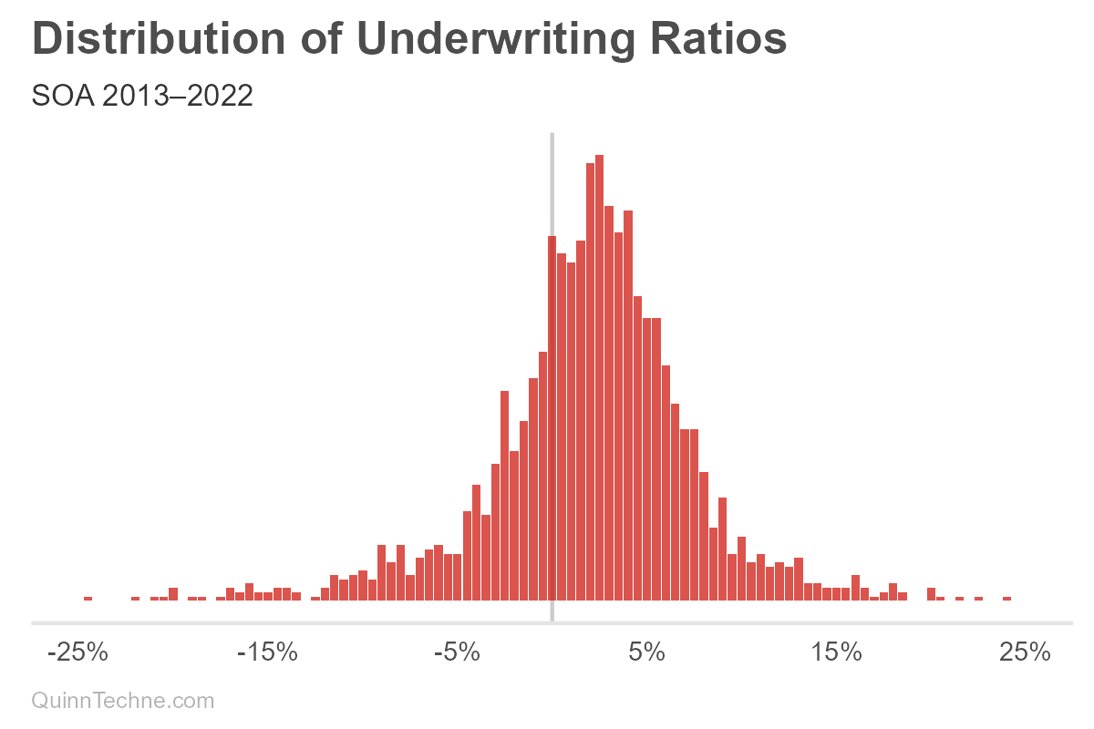
Okay, a histogram, we're done! But why do the first two histogram steps if step three is "calculate the standard deviation"?
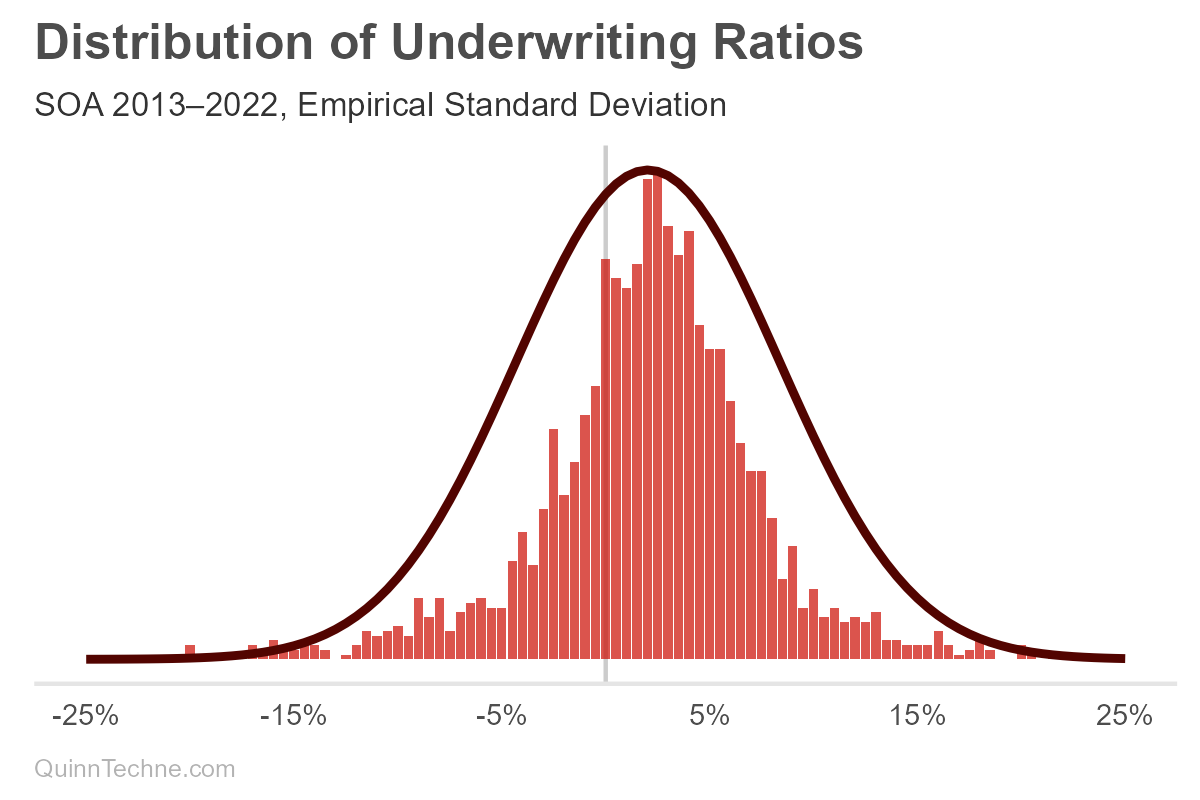
The UWR distribution seems like the MHPA data, which looks like a thinner normal distribution with wider tails. A normal distribution doesn't quite fit, as you can see in the red curve. One way to directly model this not-so-normal distribution is with a mixture of two normal distributions. However, we could also do better by decomposing and modeling the variables building up this aggregate curve, considering the causal forces behind its data-generating process.
The SOA must have noticed the odd fit, too, because their parameter fitting steps continue:
4. "The R-squared was calculated by comparing the bin frequencies to predicted normal curve frequencies."
Umm, what? R-squared is a regression analysis statistic.
So, yes, you can go into the Excel model documentation workbook and find a macro that maximizes the R-squared of normalized Gaussian probability densities, regressed on bin frequencies—which is how Cthulhu was summoned last time to reign terror on earth.
You could use a Bayesian model or Maximum Likelihood Estimation. But R-squared? The formula minimizes squared errors. This will overemphasize fitting peaks, where most observations are, at the expense of under-fitting the tails, which is dangerous if the tails are of interest—risk lives in the volatility.
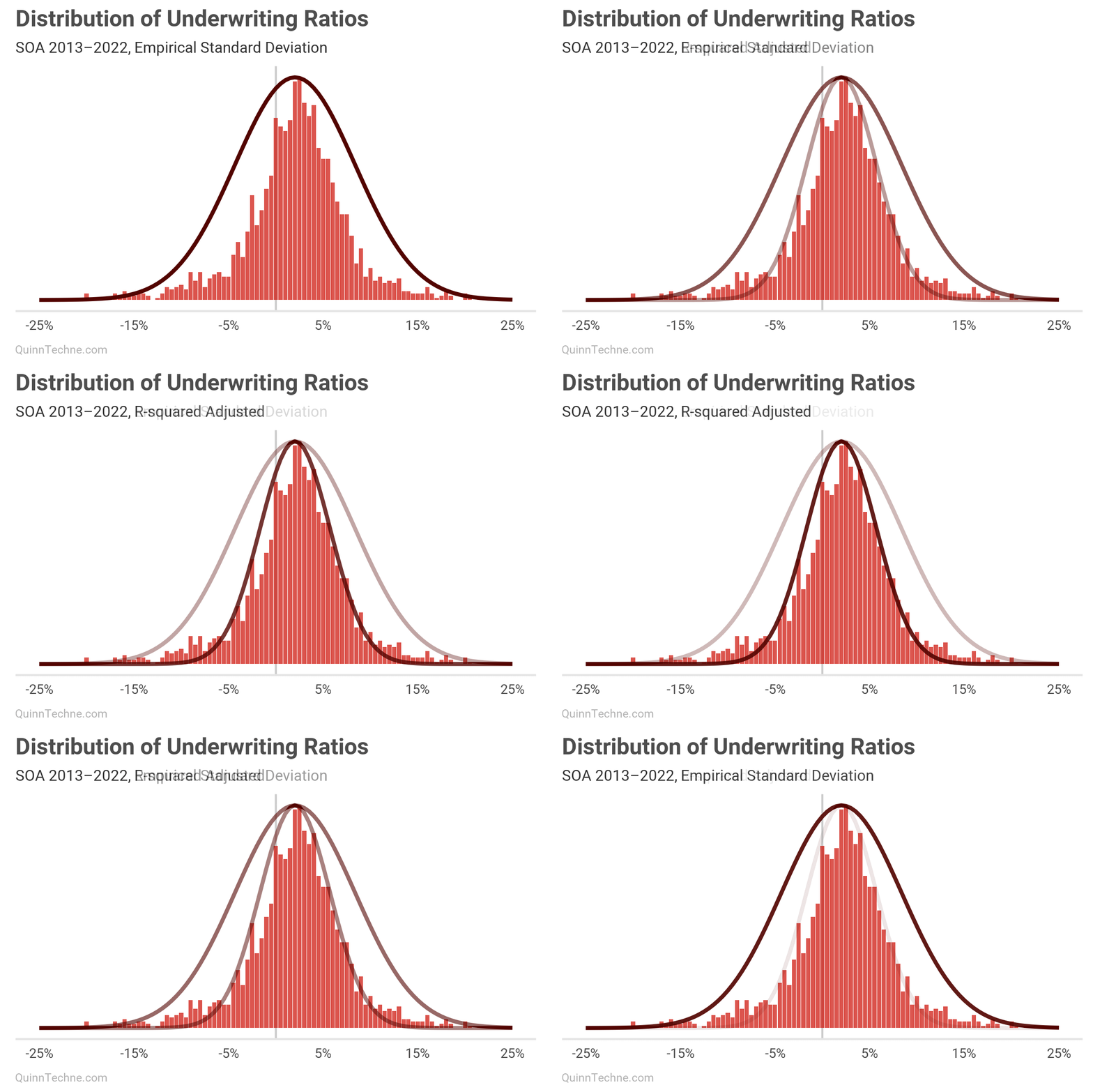
We can see that visually, this smaller SD fits the peak nicely but fails to capture the tails, as predicted.
I wrote the authors of this SOA model about the R-square method and their justification for it. They replied, "We know that our UM data points were reported by MCOs that had mix of Medicaid program types, different margin premium assumptions and various provider networks. All of these characteristics tend to overstate the variation in UM results. This supports the direction of our adjustments."
That's reasonable. In-state variation plus between-state variation will likely have more deviation than in-state variation alone. The UMG model will only be used for one state at a time; thus, the SD should be modeled with a state variable. Yet R-squared fails to do that. It accounts nowhere for a state variable.
But I know a guy who fits parameters and incorporates state variables, too.
Designing Bayesian Models
Bayesian inference is all about parameters. MHPA had a good idea to go with it. Our goal is to model the SD so that it does two things:
- Incorporates a state variable
- Has a member months component to capture reducible variation
We might consider incorporating a year variable into the SD, though the model is intended for prospective underwriting margin components. One would need to decide if UWR deviations will look like pre-COVID or if the ways state Medicaid plans adjusted to COVID will persist post-COVID. These charts show UMG statistic distributions with the COVID years in darker lines:
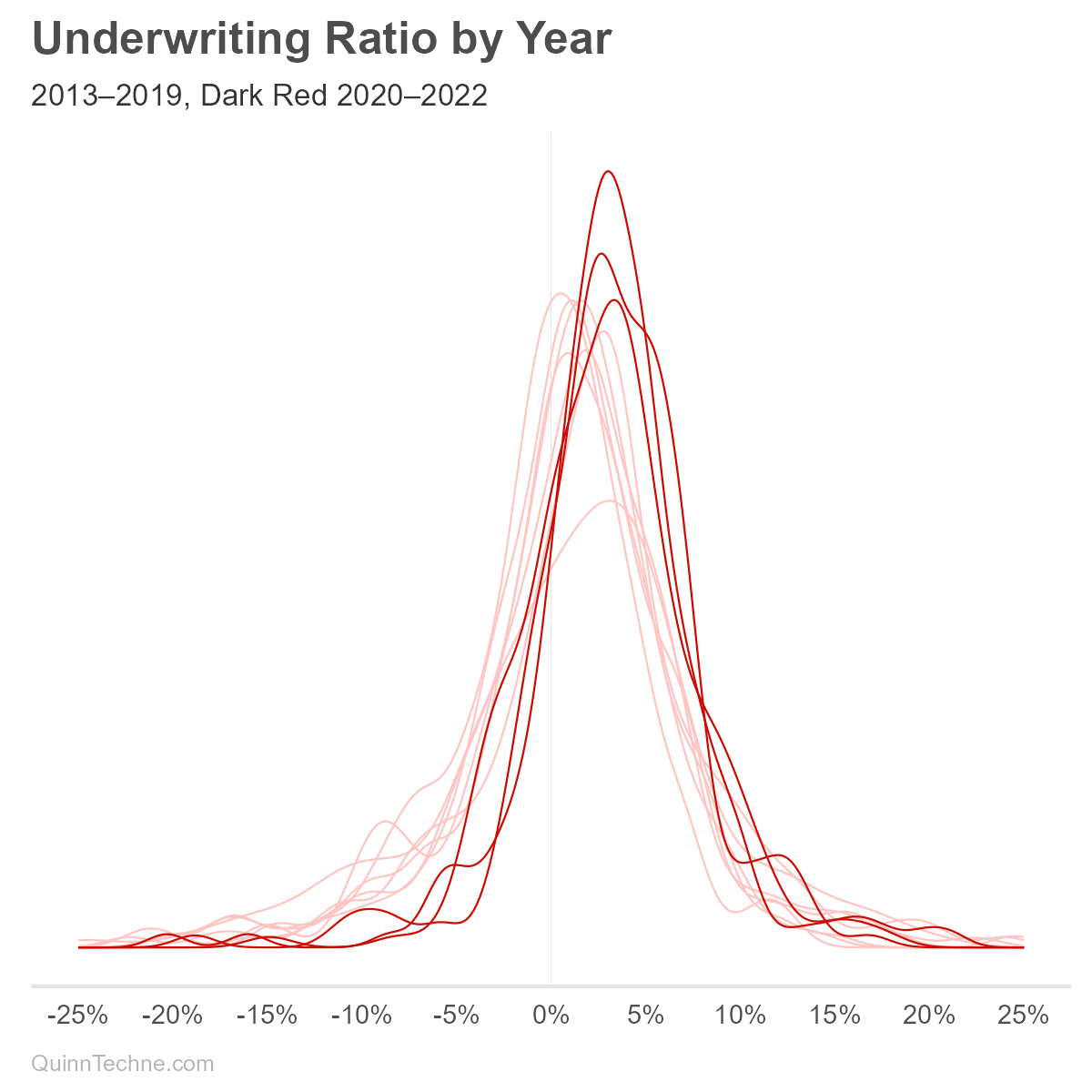
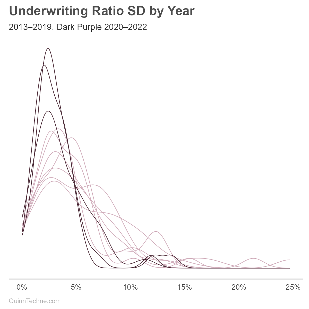
We can see from the darker lines that COVID is affecting UWR means (red) and SD (purple). The Centers for Medicare & Medicaid Services (CMS), the federal oversight of Medicaid, encouraged states to adopt risk-mitigation strategies in response to COVID. These strategies would lower the UWR SD, all else equal, because extreme higher or lower UWRs would be minimized by the risk-mitigation. Without more research, it's unclear which states implemented or maintained these strategies. We'll use all years of data for now.
Instead of R-squared, let's build a Stan model and do some Bayesian parameter fitting. We want to model UWRs by state. We can also include the year in the means so that the UWR SD picks up less year-to-year variation. The SD itself we'll model using the irreducible and reducible alpha and omega like MHPA, but state-specific. Last, we'll make this a multi-level (or hierarchal) model where mu (the average UWR, not the SD), alpha, and omega draw from a population parameter, sometimes called a hyperparameter, or a grand parameter in this case. This multi-level approach works well for states with few data points but does require tracking layers of parameters. Just like the movie Inception!
The multi-level model is a model with memory. As each state, year, or MCO is fit, it updates the distribution from which all others draw. Without this population layer, every local state, year, or MCO layer would fit without knowledge of the others. It would be like modeling with amnesia. The benefit of having memory is that it regularizes the model. Small samples or variables with a lot of spread get pulled toward, or weighted, with the population. This is known as partial-pooling.
We will build a series of models from low to high complexity:
- Force the parameters to mimic the R-squared values.
- Use the MHPA formulation without states.
- Expand the No. 2 model to have multi-level state-specific parameters.
- Include an MCO variable to the multi-level model.
Model No. 1 — R-Squared
A simple model with state-specific means and a fixed SD from the SOA model. The SOA model documentation does include an "MCO Size" curve selection. That won't be modeled here, but I will bring it up again later as it mimics some of the MHPA modeling of reducible variance as member months increase.
$$\text{uwr}[n] \sim \mathcal{N}\bigl(\mu_{\text{state}[n]}, \text{soa_sigma}\bigr) \quad \text{for } n = 1, \dots, N$$
$$\mu_j \sim \mathcal{N}(0.015, 0.005) \quad \text{for } j = 1, \dots, \text{states}$$
- \(\text{uwr}[n]\): Observed underwriting ratio for observation \(n\).
- \(N\): Number of observations.
- \(\text{states}\): Number of unique states.
- \(\text{state}[n]\): State index for observation \(n\).
- \(\text{soa_sigma}\): SD, from the SOA R-squared method.
- \(\mu_j\):
mu, state-specific mean for state \(j\). The 1.5% ± 0.5% prior is weakly informative from what was seen in Part I.
A note on priors: all probability is conditional probability. Whatever the topic, you have some background information about it. It's like breathing, and you forget about it until you hold your breath. I can control my breathing! I do have background information if I stop and think about it!
Bayesian priors are how you encode that background information. In cases where sample sizes are small or offer little new information, because they're highly varied, the prior plays a larger role in the output. It can even handle no samples. In the absence of data, the posterior distribution equals the prior. The prior takes its full value.
Earlier, I mentioned missing data with a California example. The prior will still be updated by the available six observations, but not as much updating as Florida gets with 99 observations. The starting prior 1.50% ± 0.50% updates into a normal posterior distribution of mu for California: 1.55% ± 0.48%, and Florida: 0.98% ± 0.29%.
Stan model code:
data {
  int <lower = 1> N;
  int <lower = 1> states;
  array [N] int  <lower = 1, upper = states> state;
  real <lower = 0> soa_sigma;
  vector [N] uwr;
}

parameters {
  vector[states] mu;
}

model {
  mu ~ normal(0.015, 0.005);

  for (n in 1:N){
    uwr[n] ~ normal(mu[state[n]], soa_sigma);
  }
}

generated quantities {
  vector[N] y_rep;
  vector[N] log_lik;

  for (n in 1:N) {
    y_rep[n] = normal_rng(mu[state[n]], soa_sigma);
    log_lik[n] = normal_lpdf(uwr[n] | mu[state[n]], soa_sigma);
  }
}
The data list is set up once with all variables needed in subsequent models.
### Stan compile
mod_check <- cmdstan_model(stan_code_r_squared, compile = FALSE)
mod_check$check_syntax()
stan_mod_r_squared <- cmdstan_model(stan_code_r_squared, pedantic = TRUE, dir = 'c:\\system_specific')

### Stan input
stan_mod_list_r_squared <- list(
  N = nrow(soa_data),
  states = length(unique(soa_data$state)),
  years = length(unique(soa_data$year)),
  mcos = length(unique(soa_data$snl_statutory_entity_key)),
  state = as.numeric(factor(soa_data$state)),
  year = as.numeric(factor(soa_data$year)),
  uwr = soa_data$uw_ratio,
  member_months = soa_data$member_months,
  mco = as.numeric(factor(soa_data$snl_statutory_entity_key)),
  soa_sigma = 0.0362 # 2013-2022
)

### Stan Fit
stan_fit_r_squared <- stan_mod_r_squared$sample(
  data = stan_mod_list_r_squared,
  set.seed(20250313),
  iter_warmup = 1000,
  iter_sampling = 1000)
Model No. 2 — MHPA-Style
A model with state-year-specific means and SD with inputs from alpha and omega with the latter scaled by member months.
$$\text{uwr}[n] \sim \mathcal{N}\bigl(\mu_{\text{state}[n], \text{year}[n]}, \sigma_n\bigr) \quad \text{for } n = 1, \dots, N$$
$$\mu_{j,k} \sim \mathcal{N}(0.015, 0.005) \quad \text{for } j = 1, \dots, \text{states}; k = 1, \dots, \text{years}$$
$$\sigma_n = \sqrt{\alpha + \frac{\omega}{\text{member_months}[n]}}$$
$$\alpha \sim \mathcal{N}(0.0008, 0.0002)$$
$$\omega \sim \mathcal{N}(957, 254)$$
- \(N\): Number of observations.
- \(\text{uwr}[n]\): Observed underwriting ratio for observation \(n\).
- \(\text{states}\): Number of unique states.
- \(\text{years}\): Number of unique years.
- \(\text{state}[n]\): State index for observation \(n\).
- \(\text{year}[n]\): Year index for observation \(n\).
- \(\mu_{j,k}\): Mean underwriting ratio specific to state \(j\) and year \(k\).
- \(\alpha\): Irreducible variance parameter,
alpha. It is using the Part I results as a prior. - \(\omega\): Reducible variance parameter,
omega. It is using the Part I results as a prior. - \(\text{member_months}[n]\): Exposure in member months for observation \(n\).
- \(\sigma_n\): SD for observation \(n\) composed from
alphaandomega. This is our variable of interest. Recall that the square root of the variance is SD.
data {
  int <lower = 1> N;
  int <lower = 1> states;
  int <lower = 1> years;
  array[N] int <lower = 1, upper = states> state;
  array[N] int <lower = 1, upper = years> year;
  vector[N] uwr;
  vector <lower = 1> [N] member_months;
}

parameters {
  matrix[states, years] mu;
  real <lower = 0> alpha;
  real <lower = 0> omega;
}

transformed parameters {
  vector[N] sigma;
  for (n in 1:N) {
    sigma[n] = sqrt(alpha + omega / member_months[n]);
  }
}

model {
  to_vector(mu) ~ normal(0.015, 0.005);

  //alpha ~ uniform(0.0, 10000);
  //omega ~ uniform(0.0, 10000);
  alpha ~ normal(0.0008, 0.0002);
  omega ~ normal(957, 254);

  for (n in 1:N) {
    uwr[n] ~ normal(mu[state[n], year[n]], sigma[n]);
  }
}

generated quantities {
  vector[N] y_rep;
  vector[N] log_lik;
  for (n in 1:N) {
    y_rep[n] = normal_rng(mu[state[n], year[n]], sigma[n]);
    log_lik[n] = normal_lpdf(uwr[n] | mu[state[n], year[n]], sigma[n]);
  }
}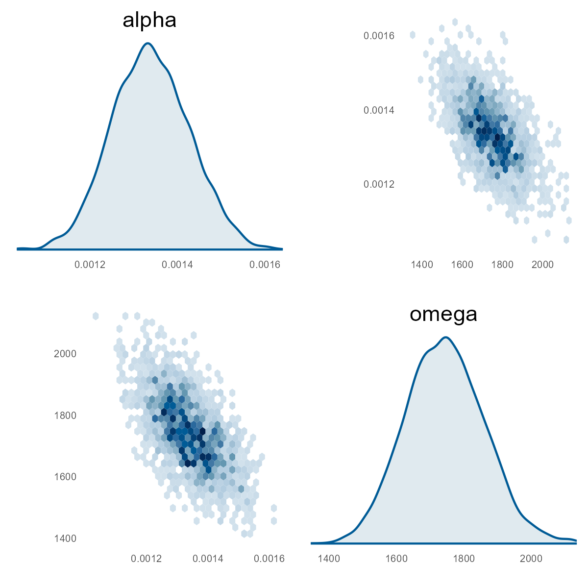
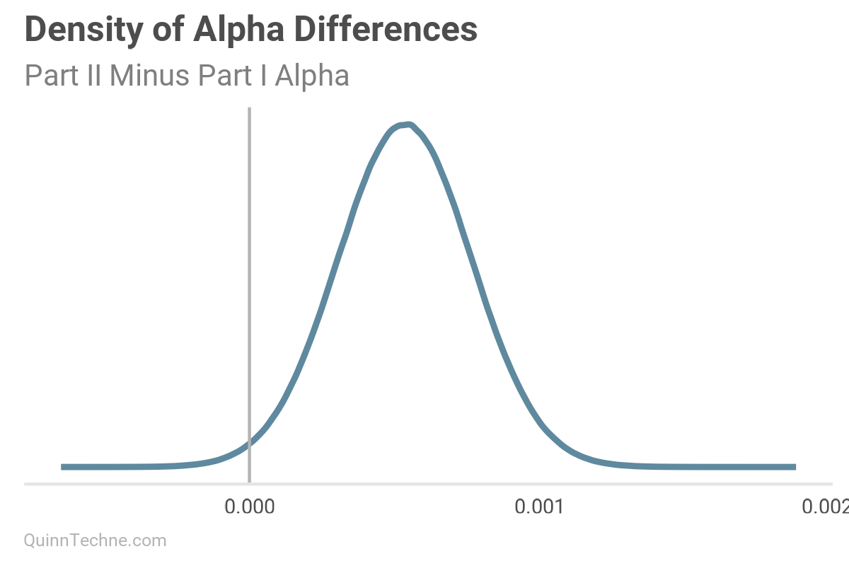
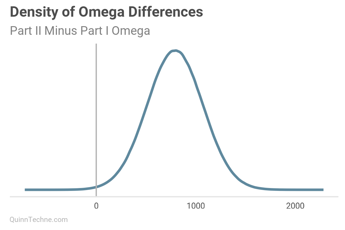
This chart is the current model's pairs plot. We used the Part I results from our MHPA Replication model as priors for this model. With more years of data, the alpha and omega parameters have noticeably increased after Bayesian updating on this data (see next two charts). It will take more member months to reduce sigma to the same size as the Part I replication model, all else equal.
Model No. 3 — State-specific Parameters
A hierarchical model decomposing both means and SD into state-level and year-level offsets around a grand mean and variance parameters.
I use the term "grand" to refer to the population level. Then, variables like state, year, or MCO offset that grand value. Suppose you wanted to model a random state; then, you could omit the state-specific offset and still get a value for your parameter—be it the mean or SD of UWR.
The catalyst for these models was to account for state variation. Multi-level models partial pool. If you have background information about a state that makes it a poor candidate to be pooled with a grand mean, you can encode a stronger priors for just that state.
Some values are on the natural log scale, like alpha and omega, because they are inside a square root, and this is one way to keep them positive. Another option, shown in the code, is to truncate draws from the prior. For example, T[0,] restricts the drawing to positive values.
$$\text{uwr}[n] \sim \mathcal{N}\bigl(\mu_n, \sigma_n\bigr) \quad \text{for } n = 1, \dots, N$$
$$\mu_n = \text{grand_mu} + \text{year_offset_mu}[\text{year}[n]] + \text{state_offset_mu}[\text{state}[n]]$$
$$\text{grand_mu} \sim \mathcal{N}(0.015, 0.003)$$
$$\text{year_offset_mu}[y] \sim \mathcal{N}(0, \text{year_offset_mu_sigma}) \quad \text{for } y = 1,\dots,\text{years}$$
$$\text{year_offset_mu_sigma} \sim \mathcal{N}^+(0, 0.010)$$
$$\text{state_offset_mu}[s] \sim \mathcal{N}(0, \text{state_offset_mu_sigma}) \quad \text{for } s = 1,\dots,\text{states}$$
$$\text{state_offset_mu_sigma} \sim \mathcal{N}^+(0, 0.015)$$
$$\sigma_n = \sqrt{\alpha_{\text{state}[n]} + \frac{\omega_{\text{state}[n]}}{\text{member_months}[n]}}$$
$$\alpha[s] = \exp(\text{log_grand_alpha} + \text{log_state_offset_alpha}[s])$$
$$\text{log_grand_alpha} \sim \mathcal{N}\left(\log(0.0008), 0.5\right)$$
$$\text{log_state_offset_alpha}[s] \sim \mathcal{N}(\text{log_state_offset_alpha_mu}, \text{state_offset_alpha_sigma})$$
$$\text{log_state_offset_alpha_mu} \sim \mathcal{N}(0, 1)$$
$$\text{state_offset_alpha_sigma} \sim \mathcal{N}^+(0, 1)$$
$$\omega[s] = \exp(\text{log_grand_omega} + \text{log_state_offset_omega}[s])$$
$$\text{log_grand_omega} \sim \mathcal{N}\left(\log(957), 0.3\right)$$
$$\text{log_state_offset_omega}[s] \sim \mathcal{N}(\text{log_state_offset_omega_mu}, \text{state_offset_omega_sigma})$$
$$\text{log_state_offset_omega_mu} \sim \mathcal{N}(0, 1)$$
$$\text{state_offset_omega_sigma} \sim \mathcal{N}^+(0, 1)$$
- \(N\): Number of observations.
- \(\text{uwr}[n]\): Observed underwriting ratio for observation \(n\).
- \(\mu_n\): Observation-specific mean underwriting ratio.
- \(\sigma_n\): Observation-specific SD derived from state-level variance components.
- \(\text{grand_mu}\): Overall, population, or (grand) mean underwriting ratio.
- \(\text{year_offset_mu}[y]\): Year-specific offset from grand mean for year \(y\).
- \(\text{state_offset_mu}[s]\): State-specific offset from grand mean for state \(s\).
- \(\alpha[s]\): State-specific irreducible variance parameter for state \(s\). Note the use of the log scale as one way to keep
alphaandomegapositive. - \(\omega[s]\): State-specific reducible variance parameter for state \(s\).
- \(\text{member_months}[n]\): Exposure in member months for observation \(n\).
Hierarchical prior SDs with \(\mathcal{N}^+\) denote truncated normal distributions. They are constrained to draw only positive values.
data {
  int <lower = 1> N;
  int <lower = 1> states;
  int <lower = 1> years;
  array[N] int <lower = 1, upper = states> state;
  array[N] int <lower = 1, upper = years> year;
  vector[N] uwr;
  vector <lower = 1> [N] member_months;
}

parameters {
  real grand_mu;
  vector[years] year_offset_mu;
  real <lower = 0> year_offset_mu_sigma;
  vector[states] state_offset_mu;
  real <lower = 0> state_offset_mu_sigma;
  real log_grand_alpha;
  vector[states] log_state_offset_alpha;
  real log_state_offset_alpha_mu;
  real <lower = 0> state_offset_alpha_sigma;
  real log_grand_omega;
  vector[states] log_state_offset_omega;
  real log_state_offset_omega_mu;
  real <lower = 0> state_offset_omega_sigma;
}

transformed parameters {
  vector[states] alpha;
  vector[states] omega;
  vector[N] mu;
  vector[N] sigma;

  for (s in 1:states) {
    alpha[s] = exp(log_grand_alpha + log_state_offset_alpha[s]);
    omega[s] = exp(log_grand_omega + log_state_offset_omega[s]);
  }

  for (n in 1:N) {
    mu[n] = grand_mu + year_offset_mu[year[n]] + state_offset_mu[state[n]];
    sigma[n] = sqrt(alpha[state[n]] + omega[state[n]] / member_months[n]);
  }
}

model {
  grand_mu ~ normal(0.015, 0.003);

  year_offset_mu ~ normal(0, year_offset_mu_sigma);
  year_offset_mu_sigma ~ normal(0, 0.01) T[0,];

  state_offset_mu ~ normal(0, state_offset_mu_sigma);
  state_offset_mu_sigma ~ normal(0, 0.015);

  log_grand_alpha ~ normal(log(0.0008), 0.5);
  log_state_offset_alpha ~ normal(log_state_offset_alpha_mu, state_offset_alpha_sigma);
  log_state_offset_alpha_mu ~ normal(0, 1);
  state_offset_alpha_sigma ~ normal(0, 1) T[0,];

  log_grand_omega ~ normal(log(957), 0.3);
  log_state_offset_omega ~ normal(log_state_offset_omega_mu, state_offset_omega_sigma);
  log_state_offset_omega_mu ~ normal(0, 1);
  state_offset_omega_sigma ~ normal(0, 1) T[0,];

  uwr ~ normal(mu, sigma);
}

generated quantities {
  vector[N] y_rep;
  vector[N] log_lik;

  for (n in 1:N) {
    y_rep[n] = normal_rng(mu[n], sigma[n]);
    log_lik[n] = normal_lpdf(uwr[n] | mu[n], sigma[n]);
  }
}
Model No. 4 — Multi-level Model
A hierarchical model decomposing both means and variances into state-level, year-level, and MCO-level offsets around a grand mean and variance parameters.
$$\text{uwr}[n] \sim \mathcal{N}\bigl(\mu_n, \sigma_n\bigr) \quad \text{for } n = 1, \dots, N$$
$$\mu_n = \text{grand_mu} + \text{year_offset_mu}[\text{year}[n]] + \text{state_offset_mu}[\text{state}[n]] + \text{mco_offset_mu}[\text{mco}[n]]$$
$$\text{grand_mu} \sim \mathcal{N}(0.015, 0.003)$$
$$\text{year_offset_mu}[y] \sim \mathcal{N}(0, \text{year_offset_mu_sigma}), \quad y = 1,\dots,\text{years}$$
$$\text{year_offset_mu_sigma} \sim \mathcal{N}^+(0, 0.01)$$
$$\text{state_offset_mu}[s] \sim \mathcal{N}(0,, \text{state_offset_mu_sigma}), \quad s = 1,\dots,\text{states}$$
$$\text{state_offset_mu_sigma} \sim \mathcal{N}^+(0, 0.015)$$
$$\text{mco_offset_mu}[m] \sim \mathcal{N}(0, \text{mco_offset_mu_sigma}), \quad m = 1,\dots,\text{mcos}$$
$$\text{mco_offset_mu_sigma} \sim \mathcal{N}^+(0, 0.015)$$
$$\sigma_n = \sqrt{\alpha_{\text{state}[n]} + \frac{\omega_{\text{state}[n]}}{\text{member_months}[n]}}$$
$$\alpha_s = \exp(\text{log_grand_alpha} + \text{log_state_offset_alpha}[s]), \quad s = 1,\dots,\text{states}$$
$$\text{log_grand_alpha} \sim \mathcal{N}\bigl(\log(0.0008), 0.5\bigr)$$
$$\text{log_state_offset_alpha}[s] \sim \mathcal{N}(\text{log_state_offset_alpha_mu}, \text{state_offset_alpha_sigma})$$
$$\text{log_state_offset_alpha_mu} \sim \mathcal{N}(0, 1)$$
$$\text{state_offset_alpha_sigma} \sim \mathcal{N}^+(0, 1)$$
$$\omega_s = \exp(\text{log_grand_omega} + \text{log_state_offset_omega}[s]), \quad s = 1,\dots,\text{states}$$
$$\text{log_grand_omega} \sim \mathcal{N}\bigl(\log(957), 0.3\bigr)$$
$$\text{log_state_offset_omega}[s] \sim \mathcal{N}(\text{log_state_offset_omega_mu}, \text{state_offset_omega_sigma})$$
$$\text{log_state_offset_omega_mu} \sim \mathcal{N}(0, 1)$$
$$\text{state_offset_omega_sigma} \sim \mathcal{N}^+(0, 1)$$
- \(N\): Number of observations.
- \(\text{uwr}[n]\): Observed underwriting ratio for observation \(n\).
- \(\mu_n\): Observation-specific mean underwriting ratio.
- \(\sigma_n\): Observation-specific SD combining irreducible and reducible variance.
- \(\text{grand_mu}\): Overall, population, or grand mean underwriting ratio.
- \(\text{year_offset_mu}[y]\): Year-specific deviation from grand mean.
- \(\text{state_offset_mu}[s]\): State-specific deviation from grand mean.
- \(\text{mco_offset_mu}[m]\): MCO-specific deviation from grand mean.
- \(\alpha_s\): Irreducible variance for state \(s\).
- \(\omega_s\): Reducible variance for state \(s\).
- \(\text{member_months}[n]\): Exposure in member months for observation \(n\).
```r
data {
  int <lower = 1> N;
  int <lower = 1> states;
  int <lower = 1> years;
  int <lower = 1> mcos;
  array[N] int <lower = 1, upper = states> state;
  array[N] int <lower = 1, upper = years> year;
  array[N] int <lower = 1, upper = mcos> mco;
  vector[N] uwr;
  vector <lower = 1> [N] member_months;
}

parameters {
  real grand_mu;
  vector[years] year_offset_mu;
  real <lower = 0> year_offset_mu_sigma;
  vector[states] state_offset_mu;
  real <lower = 0> state_offset_mu_sigma;
  vector[mcos] mco_offset_mu;
  real <lower = 0> mco_offset_mu_sigma;
  real log_grand_alpha;
  vector[states] log_state_offset_alpha;
  real log_state_offset_alpha_mu;
  real <lower = 0> state_offset_alpha_sigma;
  real log_grand_omega;
  vector[states] log_state_offset_omega;
  real log_state_offset_omega_mu;
  real <lower = 0> state_offset_omega_sigma;
}

transformed parameters {
  vector[states] alpha;
  vector[states] omega;
  vector[N] mu;
  vector[N] sigma;

  for (s in 1:states) {
    alpha[s] = exp(log_grand_alpha + log_state_offset_alpha[s]);
    omega[s] = exp(log_grand_omega + log_state_offset_omega[s]);
  }

  for (n in 1:N) {
    mu[n] = grand_mu +
            year_offset_mu[year[n]] +
            state_offset_mu[state[n]] +
            mco_offset_mu[mco[n]];
    sigma[n] = sqrt(
                 alpha[state[n]] +
                 omega[state[n]] / member_months[n]
               );
  }
}

model {
  grand_mu ~ normal(0.015, 0.003);

  year_offset_mu ~ normal(0, year_offset_mu_sigma);
  year_offset_mu_sigma ~ normal(0, 0.01) T[0,];

  state_offset_mu ~ normal(0, state_offset_mu_sigma);
  state_offset_mu_sigma ~ normal(0, 0.015);

  mco_offset_mu ~ normal(0, mco_offset_mu_sigma);
  mco_offset_mu_sigma ~ normal(0, 0.015);

  log_grand_alpha ~ normal(log(0.0008), 0.5);
  log_state_offset_alpha ~ normal(log_state_offset_alpha_mu, state_offset_alpha_sigma);
  log_state_offset_alpha_mu ~ normal(0, 1);
  state_offset_alpha_sigma ~ normal(0, 1) T[0,];

  log_grand_omega ~ normal(log(957), 0.3);
  log_state_offset_omega ~ normal(log_state_offset_omega_mu, state_offset_omega_sigma);
  log_state_offset_omega_mu ~ normal(0, 1);
  state_offset_omega_sigma ~ normal(0, 1) T[0,];

  uwr ~ normal(mu, sigma);
}

generated quantities {
  vector[N] y_rep;
  vector[N] log_lik;

  for (n in 1:N) {
    y_rep[n] = normal_rng(mu[n], sigma[n]);
    log_lik[n] = normal_lpdf(uwr[n] | mu[n], sigma[n]);
  }
}
Diagnosing Model Fits
We'll run all the models, but for this No. 4 multi-level model, let's examine more workflow details.
Before fitting the model, we'll generate samples from only our priors. This prior predictive check will help us see if we are proposing implausible draws.
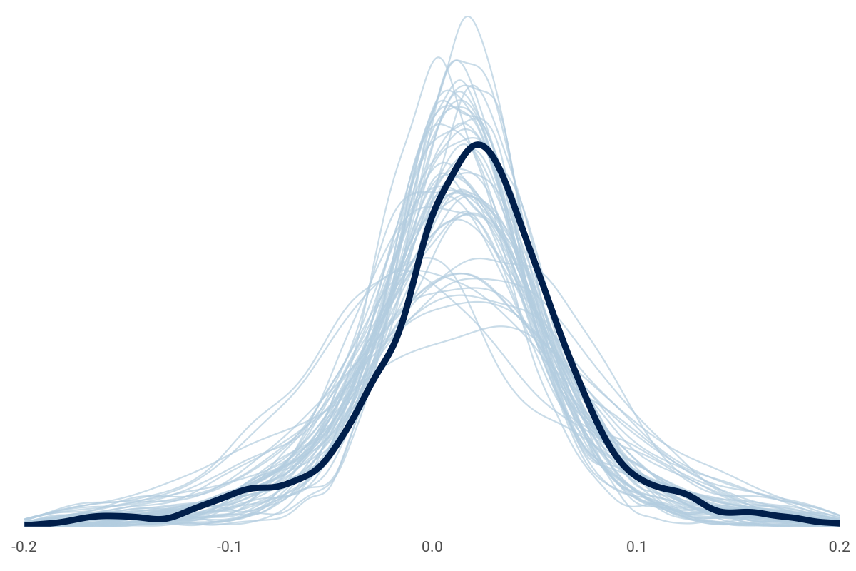
It's okay if the prior-only draws are loosely around the observations like this chart. The data will update our priors, which is something we can check here after the fitting, like this:
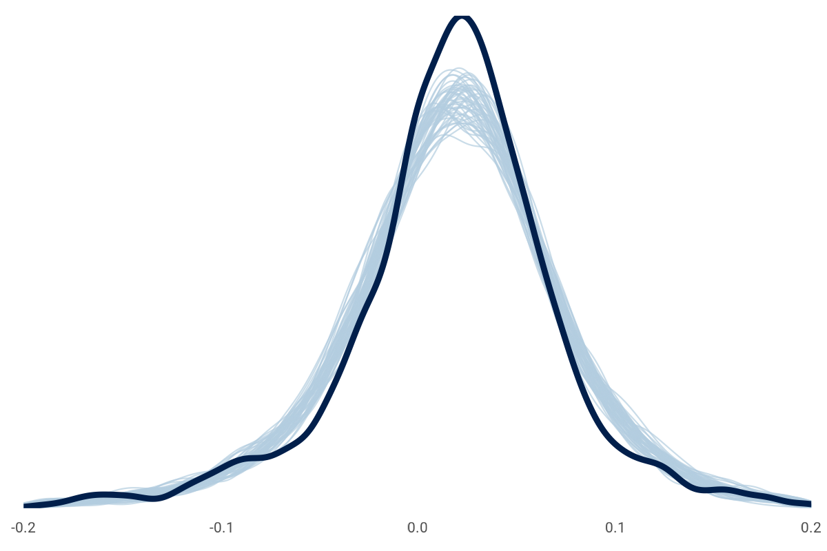
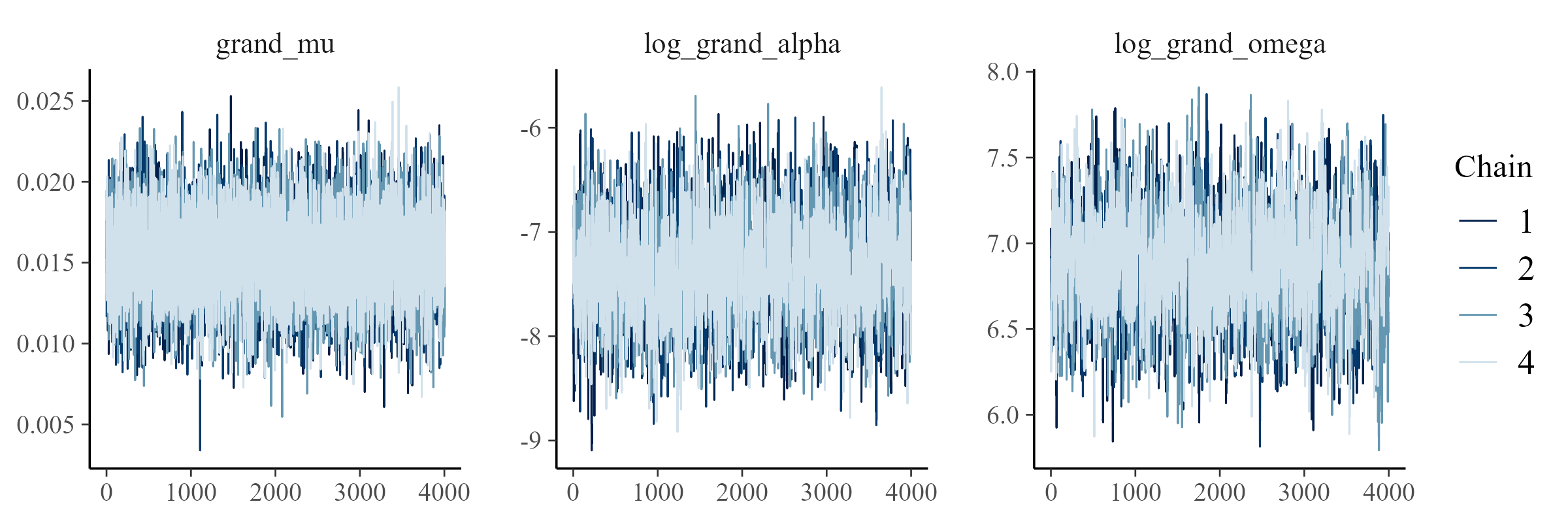
The model is fitted, and we can look at convergence diagnostics to see if our model and data fit. Among other diagnostics, a common tool is a trace plot to ensure multiple instances of the model fitting (or chains) explore the same parameter space: convergence. A related statistic is \( \hat{R} \) (pronounced "r-hat"), which we want close to 1.00. Here is an example of the \( \hat{R} \) for a subset of Model No. 4 parameters. The first 10 parameters are looking good.
> stan_fit_multi_mco$print(max_rows = 10)
 variable             mean  median    sd   mad      q5     q95 rhat   ess_bulk
 lp__              6155.30 6155.33 19.95 19.99 6122.04 6187.74 1.00     3256
 grand_mu             0.02    0.02  0.00  0.00    0.01    0.02 1.00     8303
 year_offset_mu[1]   -0.01   -0.01  0.00  0.00   -0.01    0.00 1.00     6141
 year_offset_mu[2]    0.00    0.00  0.00  0.00   -0.01    0.01 1.00     5948
 year_offset_mu[3]    0.01    0.01  0.00  0.00    0.00    0.01 1.00     5372
 year_offset_mu[4]    0.00    0.00  0.00  0.00   -0.01    0.00 1.00     5567
 year_offset_mu[5]    0.00    0.00  0.00  0.00   -0.01    0.00 1.00     5441
 year_offset_mu[6]   -0.01   -0.01  0.00  0.00   -0.01    0.00 1.00     5263
 year_offset_mu[7]   -0.02   -0.02  0.00  0.00   -0.02   -0.01 1.00     5591
 year_offset_mu[8]    0.01    0.01  0.00  0.00    0.00    0.01 1.00     5173

 # showing 10 of 8113 rows (change via 'max_rows' argument or 'cmdstanr_max_rows' option)
Here are trace plots of the grand variables in the model. This is the desired pattern. An undesired pattern would be clearly separate lines (or chains) with little overlap. To save space, I'm not going to display all the trace plots for all models and variables. It would be thousands of plots!
We can compare draws from the updated model to the observed data. This step is a follow-up to the prior predictive check. Now, we're looking at the posterior predictive distribution. We looked at charts like this in Part I. Here they are for these Part II models:
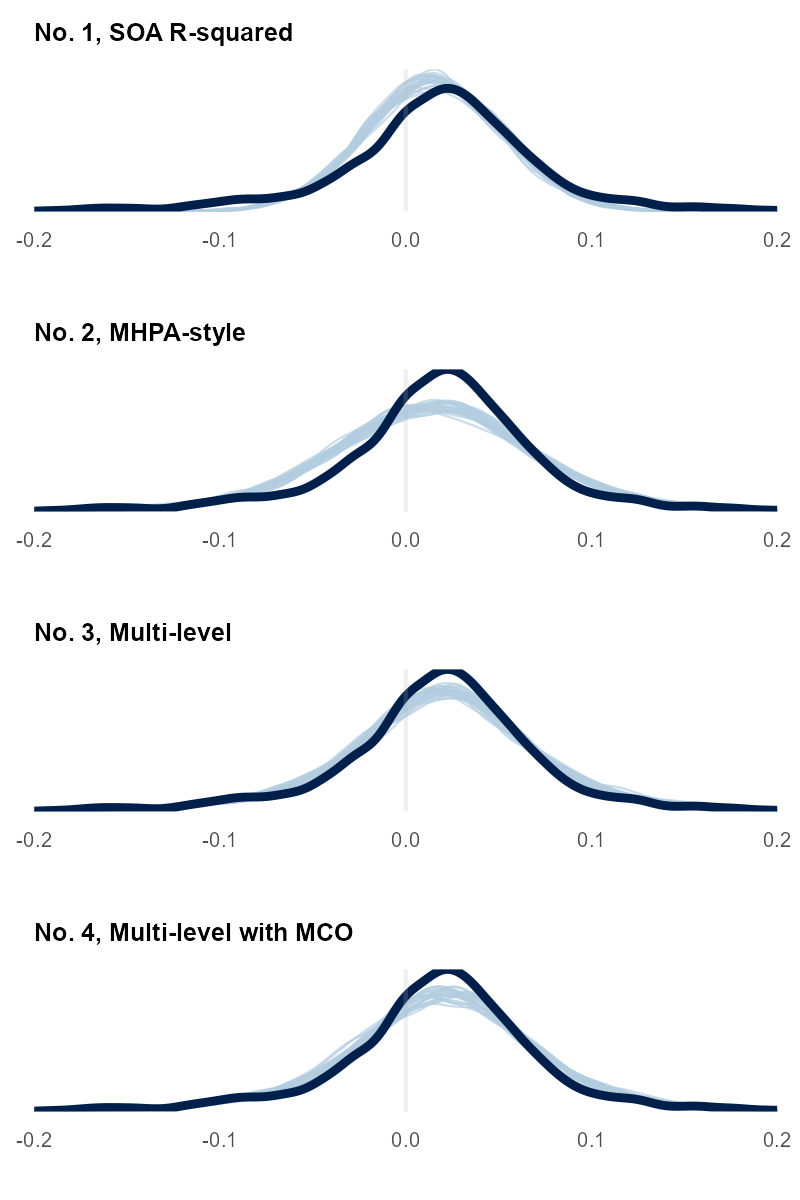
Earlier, we looked at a histogram with a red normal distribution that didn't fit the aggregate data well. It didn't match the peak and tail shape. This model includes more variables about MCO, year, and state to capture the data-generating process of the observed data.
The four charts show how more variables help our model (light blue lines) better predict the observed data (dark blue line). Each model we fit seems to do a better job, but it is hard to tell with No. 3 and No. 4. We can look at a related mathematical measure with leave-one-out cross-validation (or an approximation of it) to get a quantitative look. We also saw these statistics in Part I. We'll skip the math for today, but the gist is to approximate how likely a specific UWR would be if predicted using only the model trained on all the other data points. This leave-one-out gauges whether your model can reliably forecast never-before-seen observations or is memorizing the fitting data—overfitting.
The measure is Expected Log Predictive Density (ELPD). Higher values are desired. It is a way to check that added model complexity doesn't lead to overfitting. The output for these models looks like this:
> loo_compare(loo_list)
                   elpd_diff  se_diff
model_multi_mco         0.0       0.0 # Model No. 4 -- Relative Best by ELPD
model_multi          -127.4      15.2 # Model No. 3
model_mhpa           -456.0      41.1 # Model No. 2
model_r_squared     -1395.8     163.2 # Model No. 1
Results
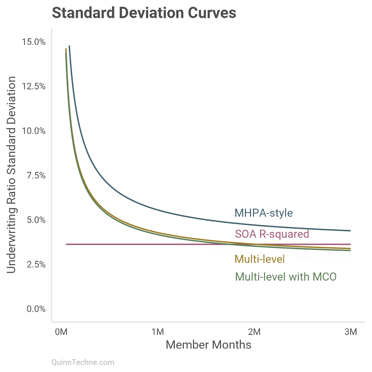
We can look at the average SD under every model as member months increase. This is similar to the chart in Part I but now with these models:
Each colored line has its distribution. Here is model No. 4 with several lines drawn from its posterior distributions to give a sense of which curves are most plausible given the model and data:
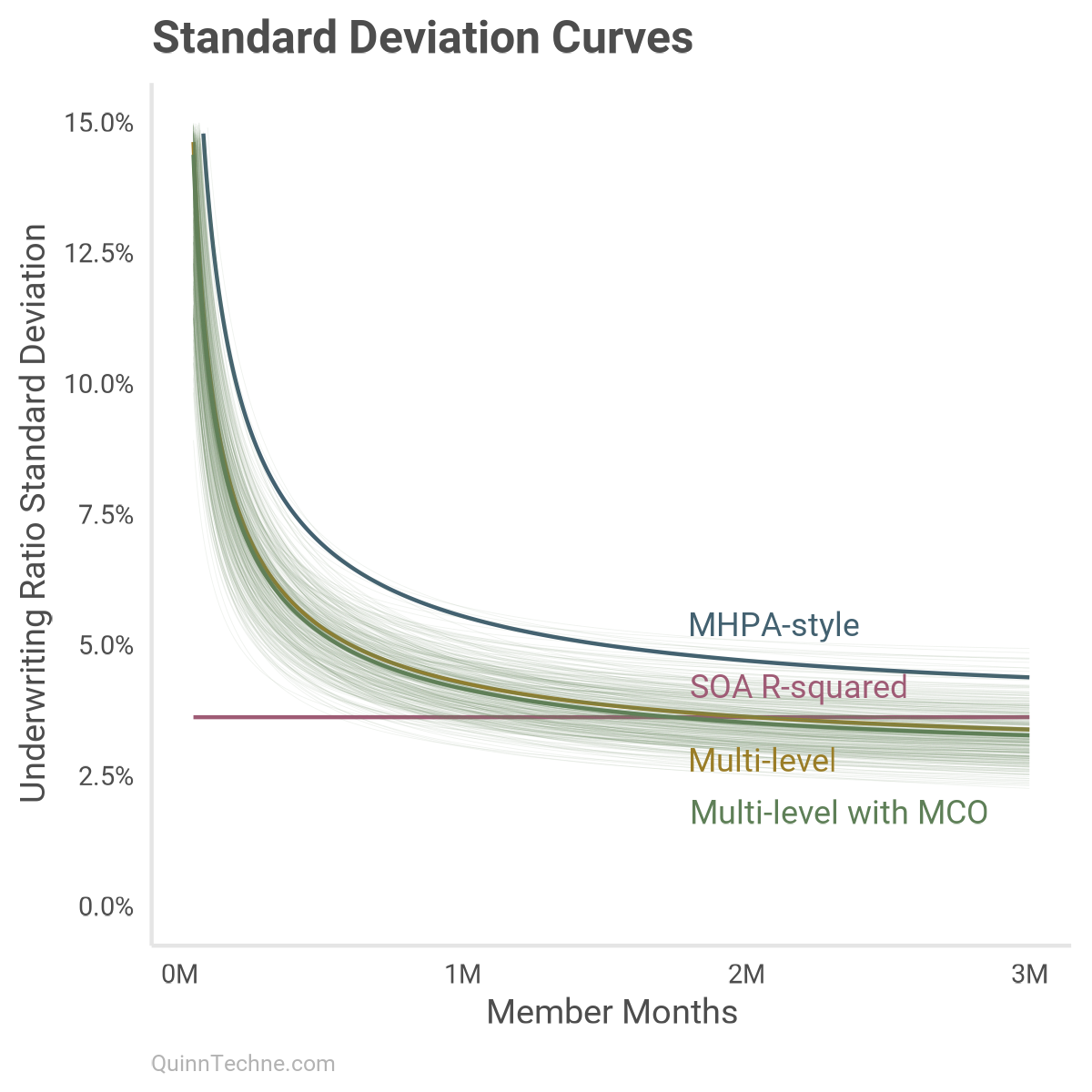
This chart shows that around one million member months, most models start to use a UWR SD in a similar probability space. By two million member months, all models are predicting a similar phenomenon with MHPA-style a little off.
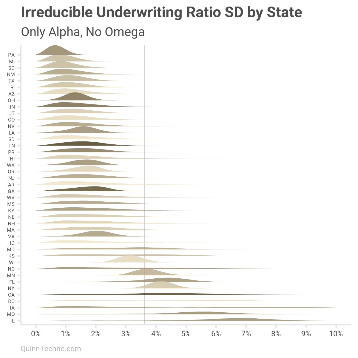
We modeled states with alpha and omega, an irreducible and reducible SD component. Here is how states' UWR SDs vary if only looking at the state-specific irreducible component alpha. You would get similar results under scenarios with large member months, millions of them. Darker colors are for states with larger median member month counts.
Moreover, about one-third of the 1,899 UWM observations are for MCOs with less than one million member months. To include member month sizes, we can re-calculate each state, adding omega scaled by states' median member months. This will be alpha plus a scaled omega specific to each state:
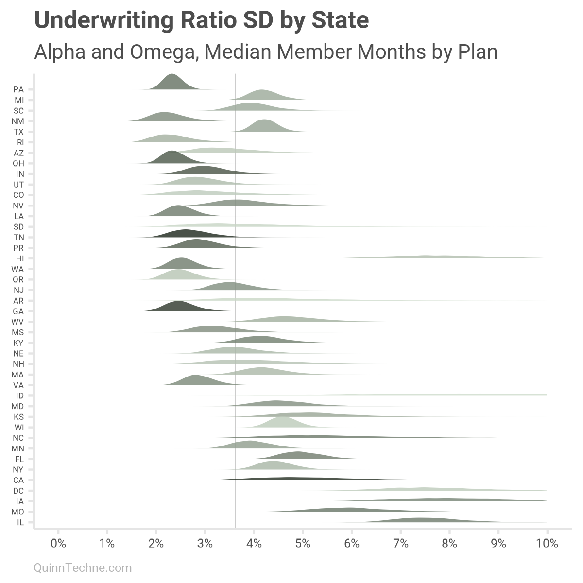
As mentioned, states with low sample sizes will have more varied parameters. Take California, for example (CA, five up from the bottom), with high median member months (darker color) but only six data points to work with. The UWR SD is flatter, and more spread out than other states. If a state has a lot of data showing a consistent pattern, then that state's UWR SD distribution would be thinner and taller, more certain.
The past two charts are also marked with a vertical line at 3.6% SD, approximately the SOA model default for the UWR SD. You can see how that number works for a few states. Yet some states are noticeably lower, and a few are much higher.
I mentioned earlier the SOA model documentation workbook has an "MCO Size" curve with details in the [PVT by Size] worksheet. I've plotted the all-years version here in dark red:
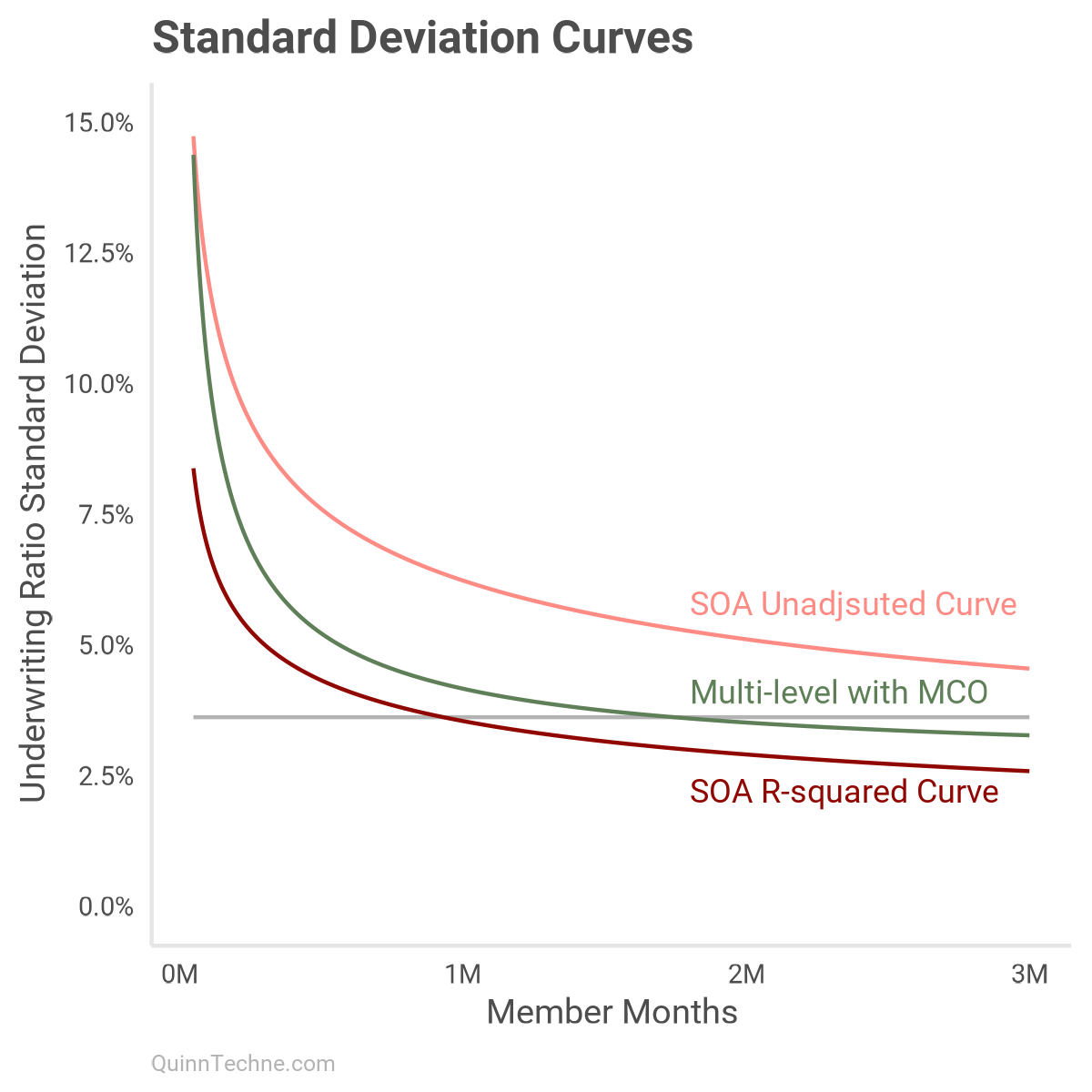
The "MCO Size" model first creates deciles by member months. Then, the UWR SD is calculated for each decile. The light red curve is fit to those empirical SDs. The R-squared adjustment then pushes the SD down to the darker version. Even as a function of member months, the R-squared adjustment undersells how much SD there is.
Taking observations on a continuous scale and discretizing them discards volatility information. Member months are on a continuous scale, and putting them into bins discards some of their volatility information. Many statistical models can handle the full complement of observations without discarding information to get bins.
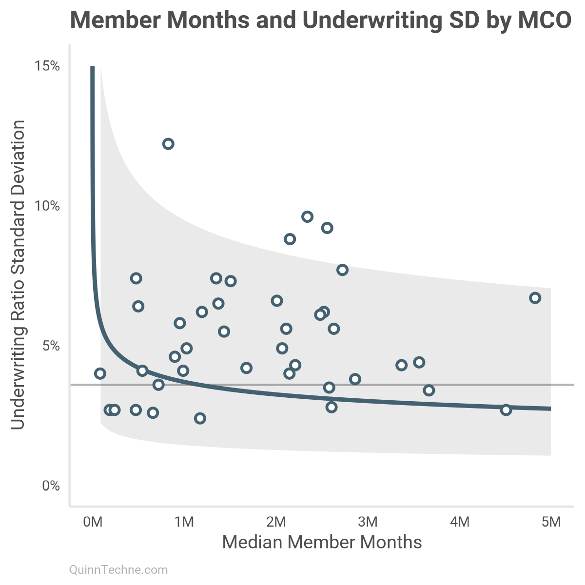
For example, this plots all MCOs with enough observations to calculate a UWR SD. Note how wide the 80% interval is, the gray ribbon. Without modeling more information, this chart suggests a range of UWR SDs 2.5%–7.5% is plausible. With more details, like the No. 4 model, that ribbon shrinks to the size of the green lines in the earlier curve plot, like 2.5%–4.0% SDs (without state offsets).
A Fitting End
I have used this SOA Underwriting Margin model and like it. It's public, transparent, and stakeholders from many backgrounds helped build it. My favorite part is that it has strong NAIC risk-based capital underpinnings. The model delivers on its intended use and I've given my justification for how to think about the UWR SD parameter fitting.
Here is what I took away from this analysis:
- First, absent state-specifics and at millions of member months, the average UWR SD parameters converge across models. However, by state, there are more differences between UWR SDs, and missing data could be playing a role. If using this SOA model, it would be worth analyzing additional sources of state-specific UMR SD data.
- Second, these Stan models show how flexible a Bayesian model can be, including the value of posterior distributions instead of point estimates as model output. The distribution of outcomes allows us to track uncertainty and enables better inference by thinking in distributions and probabilities.
- Last, if you know something about the data-generating process—you know there's a mix of Medicaid state programs that vary the UWR standard deviations—then do your best to design a model that maps your background information.
Gelman, A., Vehtari, A., Simpson, D., Margossian, C. C., Carpenter, B., Yao, Y., Kennedy, L., Gabry, J., Bürkner, P.-C., & Modrák, M. (2020). Bayesian Workflow.
arXiv:2011.01808 stat.MEstat.MEstat.ME.
Hyndman, R.J., Athanasopoulos, G. (2021). Forecasting: Principles and Practice, (3rd Edition). Otexts. https://otexts.com/fpp3/
Jaynes, E. T. (2003). Probability Theory: The Logic of Science.
Cambridge University Press. http://www.med.mcgill.ca/epidemiology/hanley/bios601/GaussianModel/JaynesProbabilityTheory.pdf
McElreath, R. (2020). Statistical Rethinking: A Bayesian Course with Examples in R and Stan (2nd Edition). Chapman and Hall/CRC. https://xcelab.net/rm/
Society of Actuaries (2024). Medicaid Underwriting Margin Model.
https://www.soa.org/4a18d1/globalassets/assets/files/resources/research-report/2024/medicaid-underwriting-margin-model.pdf
Calculations and graphics done in R version 4.3.3, with these packages:
Auguie B. (2017). gridExtra: Miscellaneous Functions for "Grid" Graphics. R package version 2.3. https://CRAN.R-project.org/package=gridExtra
Carr D, Lewin-Koh N, Maechler M, Sarkar D (2024). hexbin: Hexagonal Binning Routines. R package version 1.28.5. https://CRAN.R-project.org/package=hexbin/
Gabry J, Mahr T (2024). bayesplot: Plotting for Bayesian Models. R package version 1.11.1. https://mc-stan.org/bayesplot/
Stan Development Team (2024). cmdstanr: R Interface to CmdStan. R package version 0.7.0. https://mc-stan.org/cmdstanr/
Qiu Y (2024). showtext: Using Fonts More Easily in R Graphs. R package version 0.9-7. https://CRAN.R-project.org/package=showtext
Vehtari A, Gabry J, Magnusson M, Yao Y, Bürkner P, Paananen T, Gelman A (2024). loo: Efficient leave‑one‑out cross‑validation and WAIC for Bayesian models. R package version 2.8.0. https://mc-stan.org/loo/
Wickham H, et al. (2019). Welcome to the tidyverse. Journal of Open Source Software, 4 (43), 1686. https://doi.org/10.21105/joss.01686
Wilke C (2024). ggridges: Ridgeline Plots in 'ggplot2'. R package version 0.5.6. https://CRAN.R-project.org/package=ggridges.
Generative AIs like ChatGPT and Claude were used in parts of coding, writing, and formatting plots (Markdown with embedded LaTeX is a bit of a pain to write). Cover art was done by the author with Midjourney and GIMP.
This website reflects the author's personal exploration of ideas and methods. The views expressed are solely their own and may not represent the policies or practices of any affiliated organizations, employers, or clients. Different perspectives, goals, or constraints within teams or organizations can lead to varying appropriate methods. The information provided is for general informational purposes only and should not be construed as legal, actuarial, or professional advice.

