Time series models are like onions.
Peeling the Layers
Exponential Triple Smoothing (ETS or Additive Holt-Winters) is a time series model. It models your time series into three parts:
● Level, incorporates information from more recent observations (see Autocorrelation).
● Trend captures the pattern of change over time.
● Seasonality information from past observations that share the same periodicity.
$$ l_t = \alpha (y_t - s_{t-m}) + (1 - \alpha)(l_{t-1} + b_{t-1}) $$
$$ b_t = \beta(l_t - l_{t-1}) + (1 - \beta)b_{t-1} $$
$$ s_t = \gamma (y_t - l_{t-1} - b_{t-1}) + (1-\gamma)s_{t-m} $$
\(y_t\), observation at time t
\(l_t\), level component at time t
\(b_t\), trend component at time t
\(s_t\), seasonal component at time t
\(\alpha\), alpha, smoothing parameter for the level, takes a value of 0 to 1, where closer to 1 puts more weight on recent observations (shorter memory) and closer to 0 gives more weight to historical observations (longer memory)
\(\beta\), beta, smoothing parameter for the trend, takes a value of 0 to 1
\(\gamma\), gamma, smoothing parameter for seasonality, takes a value of 0 to 1
\(m\), periodicity of the seasonality, for example \(m = 4\) for quarterly
Only Level
Level, trend, and seasonality are layered together. Let's look at a model with only a level and add trend and seasonality next.
$$ l_t = \alpha (y_t) + (1 - \alpha)(l_{t-1}) $$
Values of \(\alpha\) closer to 1 calculate a forecast closer to recent observations, where \(\alpha\) closer to zero forecasts closer to your initial level.
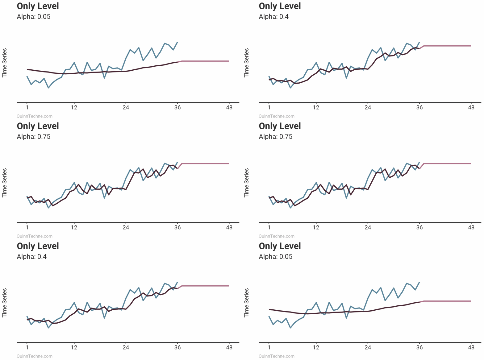
Notice how the forecast is flat. Future values only take on whatever the last level was when using a level component without trend or seasonality.
Level and Trend (Holt)
After modeling the level, trend can be layered in.
$$l_t = \alpha (y_t) + (1 - \alpha)(l_{t-1} + b_{t-1})$$
$$b_t = \beta(l_t - l_{t-1}) + (1 - \beta)b_{t-1}$$
In the first formula, the prior level \(l_{t-1}\) is adjusted by trend \(b_{t-1}\) before being compared to the current observation \(y_t\), because \(y_t\) already includes its trend.
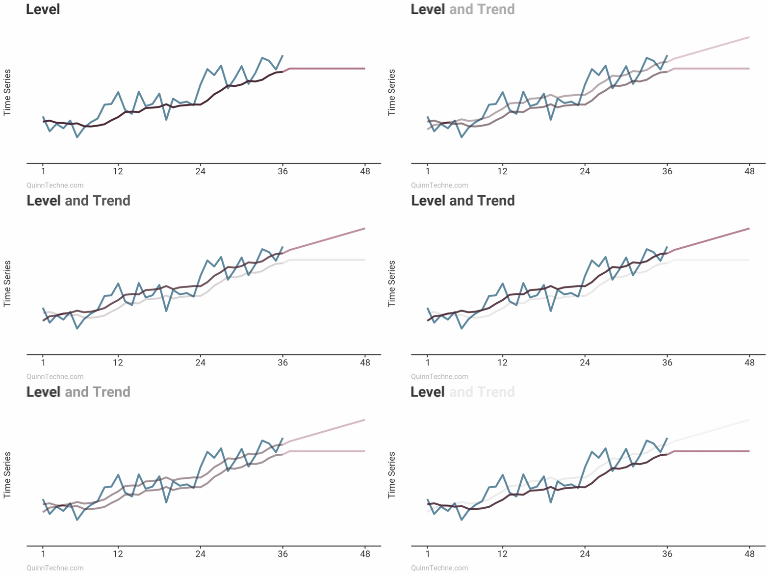
Now, the forecast begins at the last calculated levels but continues in the direction of the trend.
Level, Trend, and Seasonality (Holt-Winters)
The last layer you can include is seasonality.
$$ l_t = \alpha (y_t - s_{t-m}) + (1 - \alpha)(l_{t-1} + b_{t-1}) $$
$$ b_t = \beta(l_t - l_{t-1}) + (1 - \beta)b_{t-1} $$
$$ s_t = \gamma (y_t - l_{t-1} - b_{t-1}) + (1-\gamma)s_{t-m} $$
The intuition of \(s_t\) is that an observation stripped of level and trend is only the observation's seasonality, \((y_t - l_{t-1} - b_{t-1})\), which is then compared to the seasonal component from last time (\(m\) periods ago.)
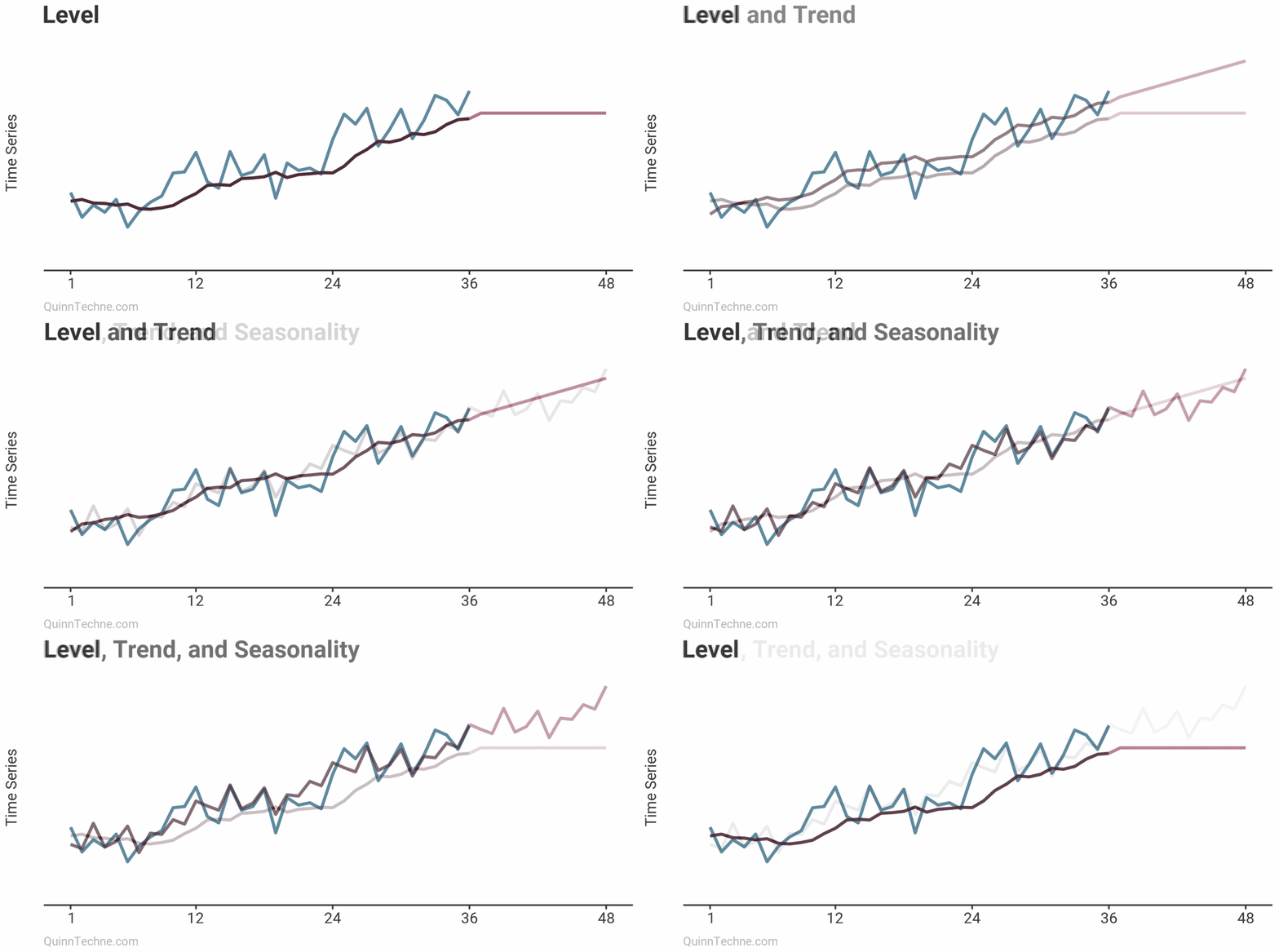
Congratulations, you've now seen the three layers of exponential smoothing for time series modeling!
Other Considerations
Exponential smoothing model parameters come in two flavors: additive or multiplicative. I've only covered additive models here. You will get similar results between the two. Still, you may find the multiplicative model useful if your seasonality or trend grows proportional to the level of growth. If your model is over-trending, the multiplicative models also offer a trend-dampening variation that may help.
Additive exponential smoothing models overlap with some ARIMA models. This understanding is useful if one is trying to decide between an ETS or ARIMA model, and they happen to be similar mathematically.
Modeling in R
The forecast package offers a useful ets() function for fitting an exponential smoothing model. You can specify if you want additive or multiplicative components. Trend or seasonality components are optional. You can also input custom smoothing parameters and let the algorithm optimize the remaining ones. The code example below introduces a function's library the first time it is used (look for the library::function).
library(forecast)
time_series_data <- 1:36 * 0.05 # Mock data

forecast::ets(
 y = time_series_data,
 model = "AAN", # Additive level and trend, no seasonality
 alpha = 0.30 # Custom alpha level smoothing parameter
)

## ETS(A,A,N)

## Call:
## forecast::ets(y = time_series_data, model = "AAN", alpha = 0.3)

##  Smoothing parameters:
##    alpha = 0.3
##    beta = 0.0252

##  Initial states:
##    l = 0
##    b = 0.05

##  sigma: 0

##      AIC AICc BIC
## -2475.306 -2474.015 -2468.972
The top code shows an ETS model with specifications to be additive level and trend with no seasonality. It also specifies 0.30 as the alpha (level) smoothing parameter. This next code shows an auto-fitting ETS model, where the model and parameters are chosen without user input.
fit <- ets(time_series_data) # Let the algorithm optimize parameters
fit

## ETS(M,A,N)

## Call:
## ets(y = time_series_data)

##  Smoothing parameters:
##    alpha = 0.2001
##    beta = 0.0201

##  Initial states:
##    l = 0
##    b = 0.05

##  sigma: 0

##      AIC AICc BIC
## -2479.695 -2477.695 -2471.777

forecast::forecast(fit, h = 3)
## Point Forecast Lo 80 Hi 80 Lo 95 Hi 95
##           1.85 1.85  1.85  1.85  1.85
##           1.90 1.90  1.90  1.90  1.90
##           1.95 1.95  1.95  1.95  1.95
The model output includes if an additive or multiplicative component was used. It also includes the smoothing parameters and initial states. If comparing models, AIC and BIC statistics are included. The forecast also gives forecast confidence intervals with the low and high bounds.
Modeling in Excel
With Excel, you have a few options for exponential smoothing. The most complex option is to use the formulas above and manually build the components. You'll understand the math well by the time you're done! Moreover, you must assume initial values and optimize parameters with Data > Solver on a loss function. Or, you can use =FORECAST.ETS.STAT() to have Excel calculate alpha (level), beta (trend), and gamma (seasonality) smoothing parameters.
For initial values, you can use the =AVERAGE() of the first few observations to initialize the level. For the initial trend, I like to use =SLOPE() (from linear regression) on all my observations. To initialize additive seasonality, subtract the =AVERAGE() of the first \(m\) observations from each of the first \(m\) observations. You are centering those first \(m\) around their mean, and will have \(m\) initial seasonality values. For example, if doing monthly seasonality, \(m\) equals 12, and you will have 12 initial seasonality values.
The medium option is =FORECAST.ETS(), which takes your time series and associated dates and automatically initializes values to make the forecast from. However, an issue is you cannot recover the initial values for level, trend, or seasonality. If you want to calculate the forecast bounds, =FORECAST.ETS.CONFINT() returns the amount to subtract and add to your forecast values to get a confidence interval.
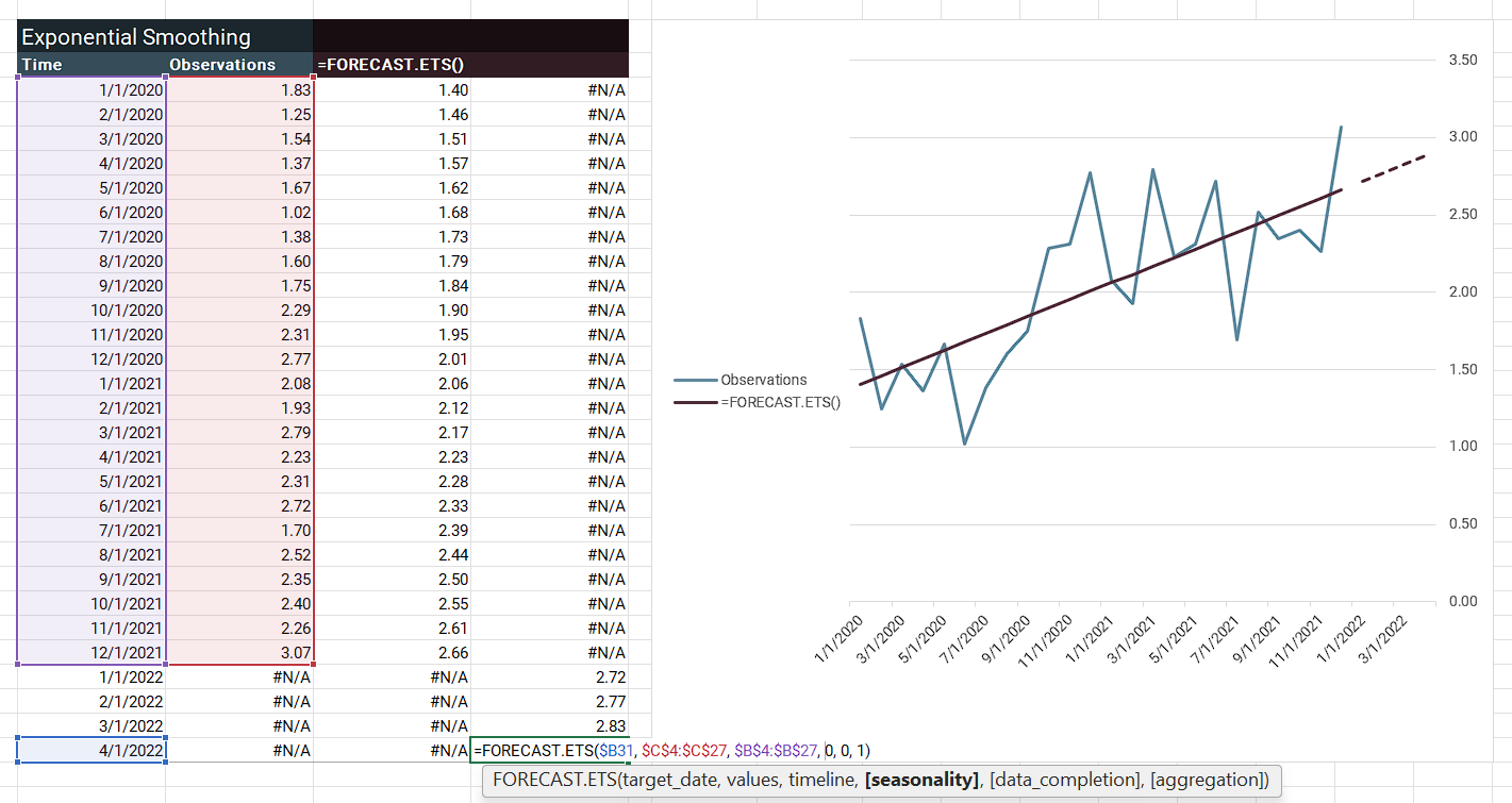
This example shows =FORECAST.ETS() on the observations. Excel is not incrementally updating the level, trend, and so forth. Instead, it has initialized values and uses the forecast formula for observed and forecasted values in the =FORECAST.ETS() column. This ETS forecast formula is for additive level and trend but no seasonality:
$$ \hat{y}_{t+h|t} = l_t + h * b_t $$
\(\hat{y}\), forecast result
\(h\), how many steps to forecast forward starting from \(t\)
Like the prior example shows, Excel has returned a line: \(y = m * x + b\), where \(b\) is your level and \(m\) is your trend.
The lightweight Excel option is to use Data > Forecast Sheet. It's =FORECAST.ETS() with the charting, forecasts, bounds, and stats built into an interface. With Forecast Sheet, like =FORECAST.ETS(), no initial values will be provided, which is too bad if you are interested in understanding what level, trend, or seasonality your model uses. Nevertheless, you will usually get a reasonable forecast.
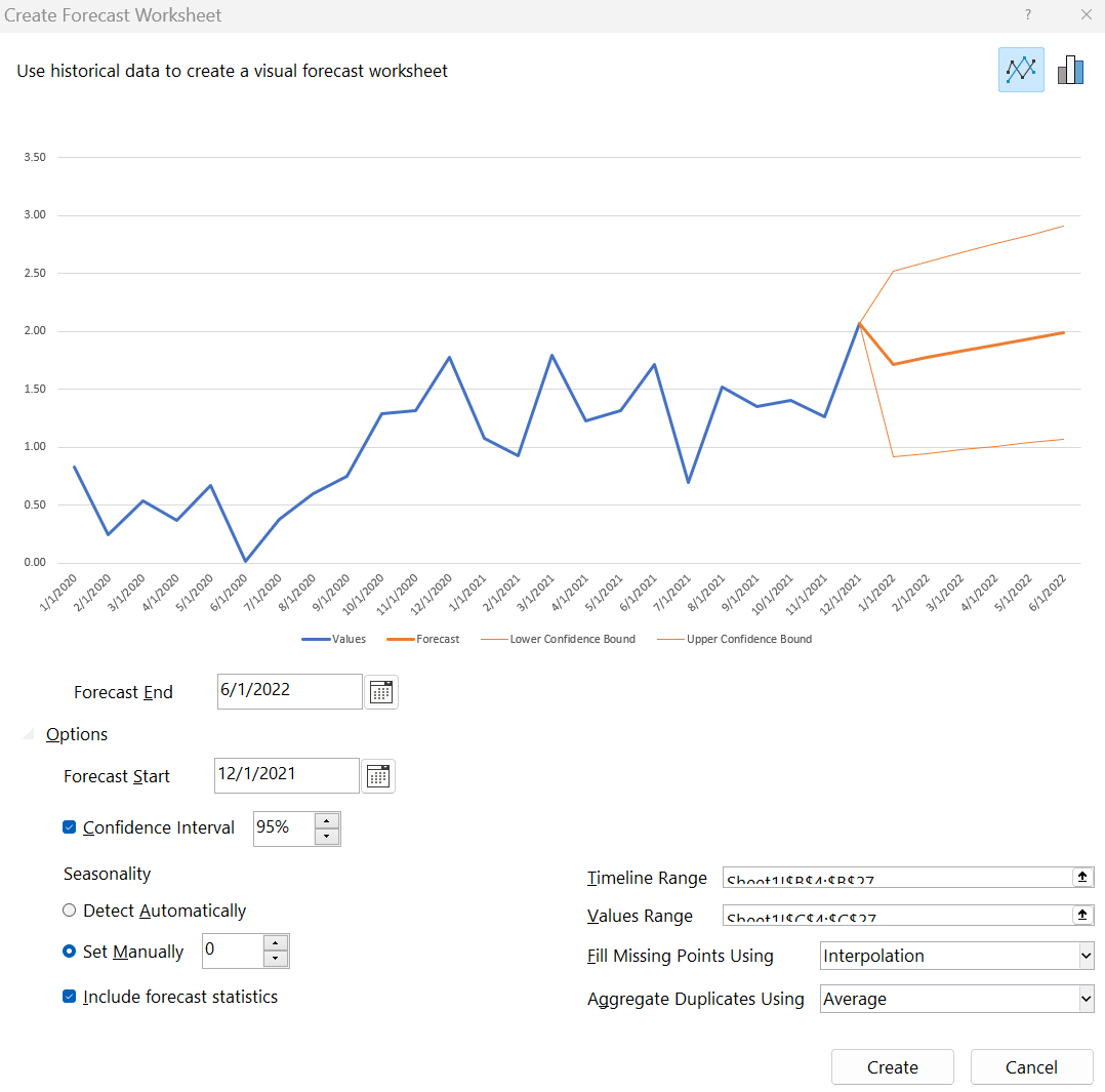
This concludes fitting exponential smoothing models to time series. Remember, this is only the model-fitting step of time series analysis. A good analysis should include exploratory data analysis, cross-validation, and post-fit diagnostics.
Hyndman, R.J. & Athanasopoulos, G. (2021). Forecasting: Principles and Practice, 3rd Edition. Otexts. https://otexts.com/fpp3/
This website reflects the author's personal exploration of ideas and methods. The views expressed are solely their own and may not represent the policies or practices of any affiliated organizations, employers, or clients. Different perspectives, goals, or constraints within teams or organizations can lead to varying appropriate methods. The information provided is for general informational purposes only and should not be construed as legal, actuarial, or professional advice.

