Cross-validation offers a modicum of solace against the tyranny of the unknown.
Why Cross-validation?
Cross-validation is a way to measure how well your model forecasts unseen observations. It also helps with balancing under or overfitting.
Under and overfitting is how your model captures the underlying patterns in the time series. Underfitting is an insipid model—too simple, whereas overfitting is a Rube Goldberg machine. It might look great on observed data but breaks down quickly in forecasts.
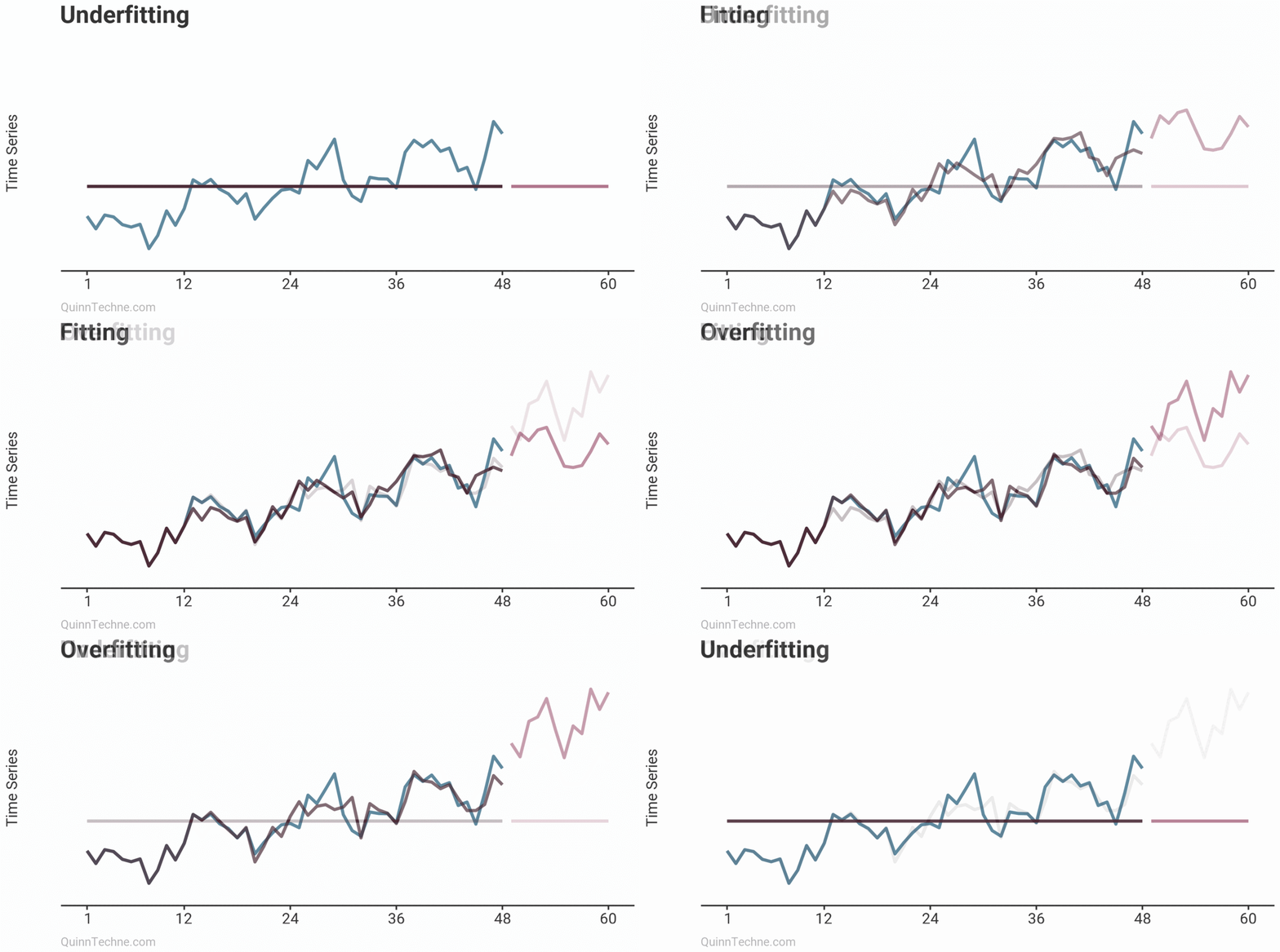
The example shows three models on the same data: Underfitting, Fitting, and Overfitting. Underfitting is the average of the observations. It does nothing to try and capture trends or seasonality patterns. The Fitting example is an ARIMA model with drift (trend) and some simple seasonality. Overfitting is also an ARIMA model but has excessive parameters. Note how well the model fits the first 24 observations. It looks impressive but comes at the cost of poor forecasts. You can already sense it's trending too quickly beyond the observed data. Later, we will see how the Fitting example ARIMA model cross-validates.
To do cross-validation, partition your data into training and testing sets. Then, build your model on the training set and see how it performs on the testing set. A model should perform reasonably on the testing data—observations unseen by the model.
Measuring Performance
Many model-fit statistics exist to measure performance on training or testing data. For cross-validation, I focus on measuring performance on the testing data. I will cover two statistics I like because they have a built-in comparison to zero.
$$ \text{Mean Absolute Error (MAE)} = \frac{1}{n} \sum_{t=1}^{n} |y_t - \hat{y}_t| $$
\(n\), number of observations being compared
\(t\), observation index
\( y_t\), the observed value at time \(t\)
\(\hat{y}_t\), the forecasted value at time \(t\)
The difference \((y_t - \hat{y}_t)\) may seem familiar because that is a residual if you recall regression models from intro stats.
$$ \text{Mean Absolute Percentage Error (MAPE)} = \frac{1}{n} \sum_{t=1}^{n} \left| \frac{y_t - \hat{y}_t}{y_t} \right| $$
MAPE is similar to MAE and is scaled by the observation \(y_t\), which makes it a unitless measure.
I mentioned liking these measures because zero is a natural baseline. However, zero can also be their weakness. If your time series data happens to include zero or near-zero values, it will undesirably influence your statistics. Imagine you go to calculate MAPE, and your observation is zero, and you divide by zero, then try to take the mean of that—#DIV/0!, anyone? If you have this problem, check out scaled errors here.
Designing Your Cross-validation
The context of your forecast will inform the design of your cross-validation. You want to understand how much data you'll usually have for training a model and how far out your forecast typically is. Because time series has a temporal element, you have to keep your data ordered and together: training followed by testing data. For example, suppose you usually have 36 months of data to forecast the next 12. Then, try to use 36 months of training data on 12 months of testing data.
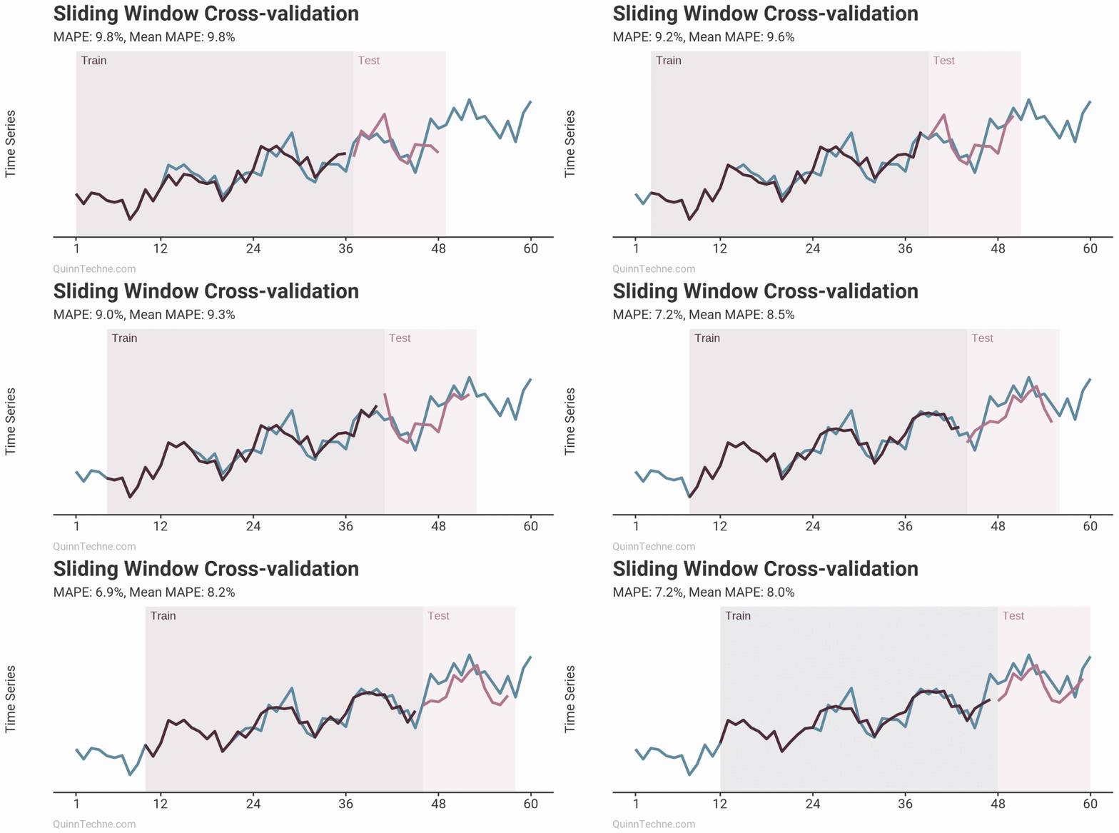
The prior example is called Sliding Window cross-validation. The number of training and testing observations remains the same for each iteration. This example shows the iteration moving forward one step each time. Because each new fitting is on data overlapping a prior fitting, the variance of the cross-validation statistics will be understated. Ideally, you have enough data to have multiple unique training and testing sets, but we cannot all be so lucky. This next chart shows the Expanding Window method.
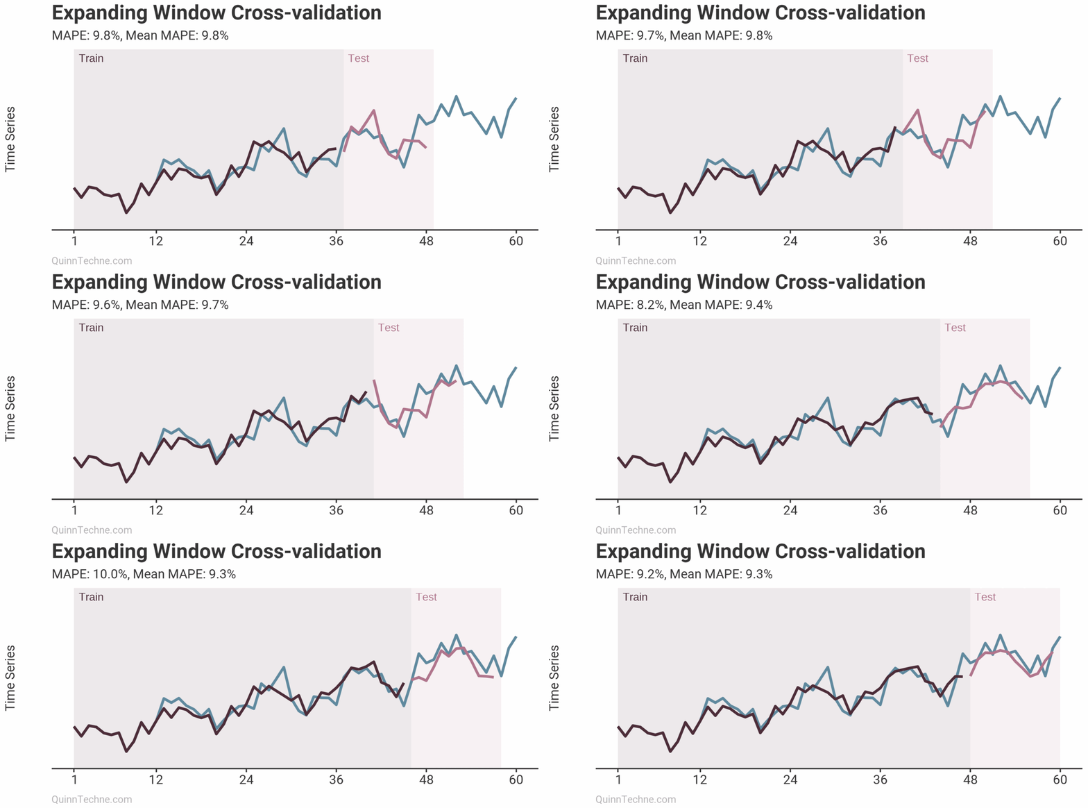
Each iteration expands the training data. It shows how the forecast performs as you add more training data. The MAPE of each iteration is shown along with the average MAPE of all iterations. Each iteration fits new model parameters, so you'll see the fit on the observed data switch sometimes. Cross-validation can test a model methodology (like the past two examples) rather than a fixed set of model parameters. More on this later.
Doing Time Series Cross-validation in R
You can build your cross-validation from first principles in R with the prior formulas and loops. This example shows one iteration of cross-validation done using the Fable package. First, you need a tsibble, a time series data frame-like object akin to tibbles from Tidyverse. This code converts an R time series object ts to a tsibble.
# Cross-validation with Fable, QuinnTechne.com
library(fable)
library(fabletools)

ts # R time series object
ts_as_tsibble <- fable::as_tsibble(ts)

ts_as_tsibble
## A tsibble: 60 x 2 [1M]
## index value
## <mth> <dbl>
## 1 0001 Jan 2.07
## 2 0001 Feb 1.47
## 3 0001 Mar 2.12
## 4 0001 Apr 2.03
Next, we'll use 48 months of the 60 observations to train an ARIMA model and look at its parameters.
ts_train <- ts_as_tsibble[1:48, ]

fit_arima <- ts_train |>
  fabletools::model(
    arima_fit = ARIMA(value ~ 1 + pdq(0,0,0) + PDQ(0,1,0))
  )

fabletools::report(fit_arima)
## Series: value
## Model: ARIMA(0,0,0)(0,1,0)[12] w/ drift

## Coefficients:
## constant
## 1.1216
## s.e. 0.1331

## sigma^2 estimated as 0.6561: log likelihood=-42.99
## AIC=89.98 AICc=90.34 BIC=93.14
Last, we'll forecast the next 12 months as our test and look at model-fit statistics.
forecast_arima <- fabletools::forecast(fit_arima, h = 12)

fabletools::accuracy(object = forecast_arima, data = ts_as_tsibble)
## A tibble: 1 × 10
## .model      .type    ME  RMSE   MAE  MPE   MAPE  MASE  RMSSE   ACF1
## <chr>       <chr> <dbl> <dbl> <dbl> <dbl> <dbl> <dbl>  <dbl>  <dbl>
## 1 arima_fit Test  0.275 0.752 0.557  3.80  8.62 0.455  0.546 -0.326

fabletools::autoplot(forecast_arima, ts_as_tsibble)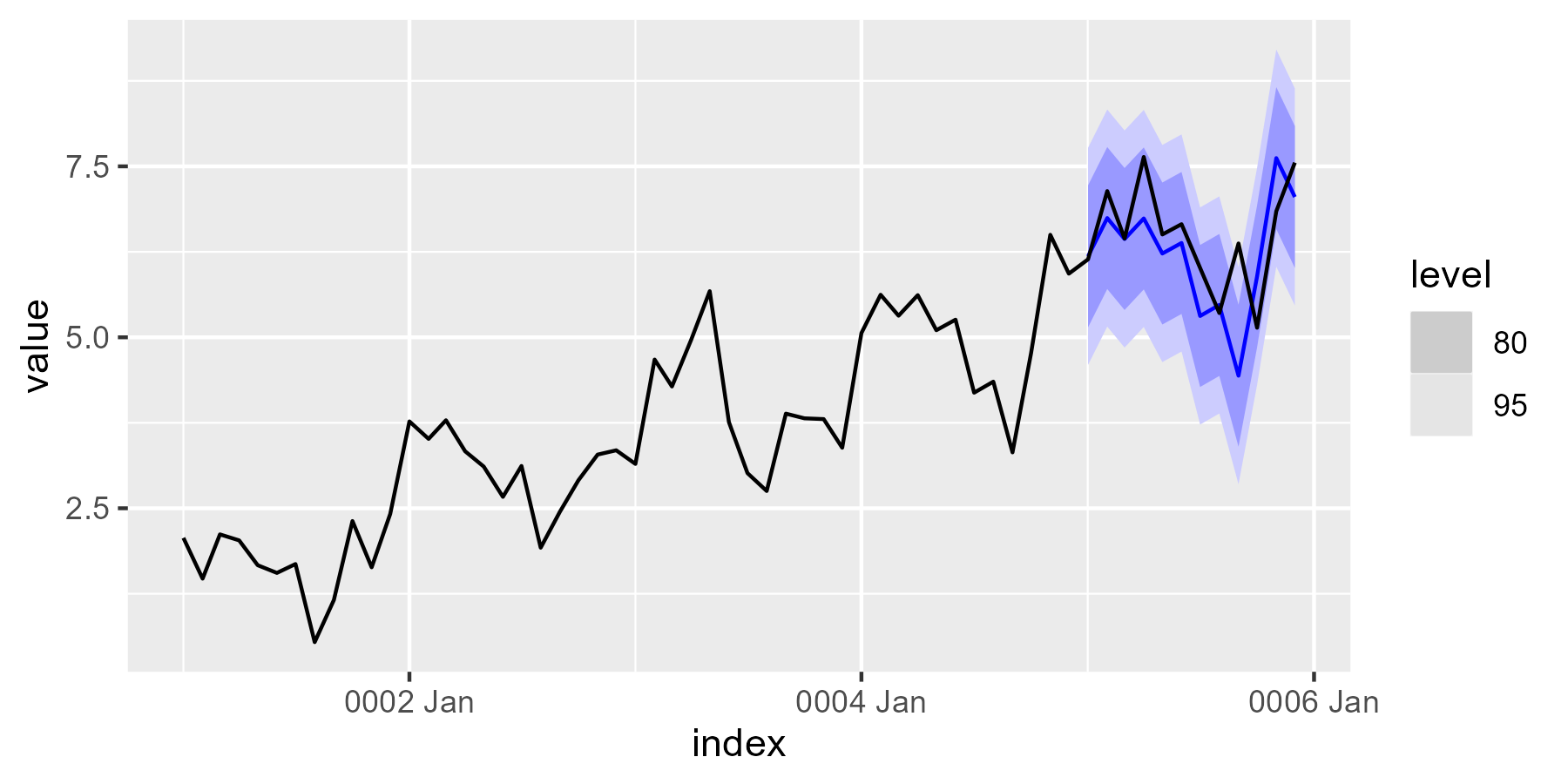
The preceding chart shows the autoplot() results of the time series and cross-validation forecast.
Doing Time Series Cross-validation in Excel
This example shows one cross-validation iteration, the same testing set as the R example. To start, array your data, fit your model (I'm using the same ARIMA model as the R example), and calculate your forecasted values. I have =NA() in several cells to help with the chart, and a freeze frame only shows the bottom of the table.
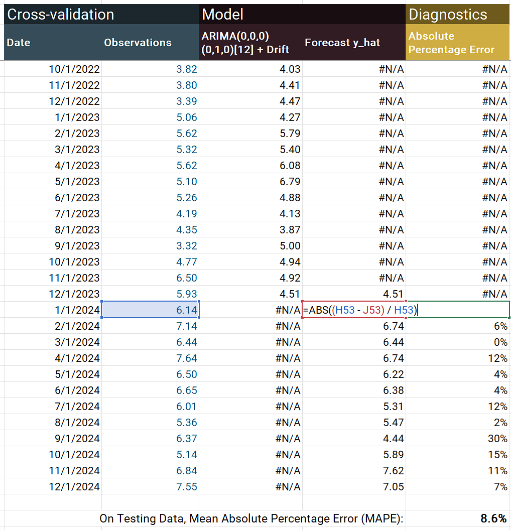
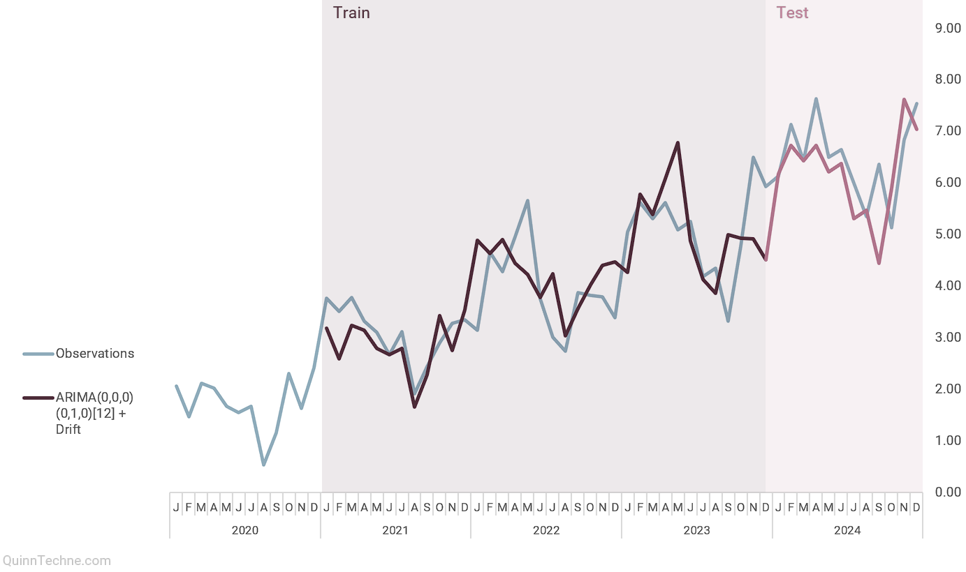
Next, calculate your model-fit statistic. In the screenshot, the opened formula shows the calculation for absolute percentage error (the APE part of MAPE). The =AVERAGE() of the APE values gives you MAPE. The MAPE statistic is calculated on the testing block of the charted data.
If iterating cross-validations in Excel, you may need custom tools or Excel VBA code. Other software, like R or Python, will have more tools for time series cross-validation.
What's Next?
You've done cross-validation, and the model-fit statistics are discouraging. Now what? You may consider a different model. However, sometimes, series are too noisy to forecast, regardless of the model or skill of the forecaster. Exploratory Data Analysis (EDA) of your time series can give you measures that indicate how difficult it might be to forecast the observed time series.
Alternatively, what if the model-fit statistics are promising? Cross-validation is like testing a method instead of testing a set of model parameters. For example, suppose I used an additive ETS model in cross-validation, and it performed well. In that case, I'll fit a new additive ETS model to all my data for my real forecast instead of using some mixture of the smoothing parameters from the cross-validation models.
If your cross-validation checks out, take solace and fit your full model.
Hyndman, R.J. & Athanasopoulos, G. (2021). Forecasting: Principles and Practice, 3rd Edition. Otexts. https://otexts.com/fpp3/
This website reflects the author's personal exploration of ideas and methods. The views expressed are solely their own and may not represent the policies or practices of any affiliated organizations, employers, or clients. Different perspectives, goals, or constraints within teams or organizations can lead to varying appropriate methods. The information provided is for general informational purposes only and should not be construed as legal, actuarial, or professional advice.

